The history of Spiking Neural Network

Still in progress
Statement: This article is expanded from the summary part of my undergraduate thesis. Plagiarism must be investigated.
1. Introduction
The development of artificial neural networks is a hot topic in the current academic and industrial circles. It is generally believed that neural networks today are divided into three generations 1. The first generation model is a confirmatory model, which was proposed by Warren McCulloch and mathematical logician Walter Pitts in the cooperative paper 2, and later summarized by neurologist Frank Rosenblatt as a perceptron 3. Deep artificial neural networks (ANNs) can be considered the second generation of neural networks. Compared with the first generation of neural networks, ANNs can solve the nonlinear fitting problem by increasing the number of network layers and parameters and exchanging a large amount of computation for superior learning performance. With the development of computer science, machine learning using ANNs has transitioned from shallow learning to deep learning and achieved great success. However, in fact, ANNs have gradually moved away from the biological basis of neural networks, so they cannot make a reasonable explanation of the working principle of the brain. At present, ANNs have been applied in many vertical fields, but they still lack generalization ability for a wider range of application scenarios and are not promising on the road to general artificial intelligence. Spiking Neuron Network ( SNN ) is considered to be a new generation of brain-based neural networks, namely the third generation of neural networks. In 1952, when Alan Hodgkin and Andrew Huxley studied the signal transmission mechanism of squid neurons, they obtained the operation process of neural membrane potential 4, which is now known as action potential and resting potential. Later, together with Huxley's experiment, the Hodgkin-Huxley model ( H-H model )5 was proposed. The H-H model has a good performance in the process of numerical simulation of neurons and has a high degree of coincidence with experimental data. Therefore, it has become an important research foundation of neuroscience. However, because it involves high-order nonlinear differential equations, it is very difficult to simulate numerically, and it is more difficult to deploy large-scale applications. In 1997, some scholars proposed the spiking neuron model 6 and compared it with other neural network models ( including threshold gates, and sigmoid gates ). It is proved that spiking neurons have the stronger computing power and more convenient numerical modeling capabilities while retaining the working characteristics of the nervous system. Since the 21st century, with the continuous improvement of the Backpropagation ( BP ) algorithm and the increase of computing resources, SNN has returned to the public view and become a new way of general artificial intelligence. Spiking neurons imitate the propagation mechanism of electrical signals of biological neurons to model. By recording the time of generating pulses, the rate of generating pulses, or directly using the entire pulse sequence to transmit information, they have the biological basis and time information coding complexity that traditional artificial neural networks do not have.
SNN has attracted great interest in the field of artificial intelligence and neuroscience because it can retain the real characteristics of organisms while exploring human cognitive principles and has great advantages in event-driven and energy-constrained machine learning tasks. The addition of the time dimension greatly helps the compact representation of large complex neural networks and helps to further understand the working mechanism of the human brain. At present, a variety of artificial neural network models have excellent performance in many fields, such as image processing ( represented by convolutional neural network, reinforcement learning ( represented by deep reinforcement learning ), natural language processing ( represented by long short-term memory model LSTMand gated recurrent unit GR). In contrast, SNN is still in its infancy in software simulation framework, hardware platform support, data set richness and accuracy. However, SNN has high efficiency in dealing with complex, sparse, and noisy Spatio-temporal information, and is particularly competitive on platforms with limited computing power. Lightweight is an important issue in the popularization of artificial intelligence. For the shortcomings of SNN, we urgently need to find a solution. Aiming at the problem of the high cost of training on general computing architecture, many heterogeneous computing platforms suitable for neuromorphic computing have been proposed, including TrueNorth 7 developed by IBM, Loihi 8 developed by Intel, ' Cambrian 1 ' 9developed by Chinese Academy of Sciences, and TianJic 10 developed by Tsinghua University. To facilitate learning in such networks, new learning algorithms based on varying degrees of biological likelihood have also been developed. Unsupervised learning develops the Spike Timing Dependent Plasticity ( STDP ) algorithm 11 based on Hebb's theory and Hebb's learning 12. Based on the BP algorithm, different continuous approximations of data and models are performed, and Spatio-Temporal Backpropagation ( STBP ) algorithm13 and pulse sequence convolution learning algorithm are developed.
To construct an SNN learning and inference system, four aspects need to be considered, including the encoding of data ( external stimuli ), the construction of a suitable neuron model, the formulation of learning rules, and an efficient computing platform. The coding methods mainly include rate coding and time coding, etc., which are not introduced in detail here. In the next three sections, we focus on the main models, training methods, and existing neuromorphic periods of SNN. In view of the shortcomings of existing models and training methods, a neuron model between SNN and ANNs is proposed through model fusion to adapt to artificial intelligence tasks on general computing platforms and heterogeneous computing platforms.
2. evolution of spiking Neural model
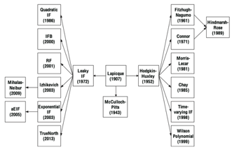
Figure 1: history
In order to study the working mechanism of the brain, neuroscientists have proposed a large number of mathematical models based on the working mode and cell structure of neuronal cells. Most of the current neuron models originated from the H-H model. The H-H model can have simulation results that are in good agreement with the experimental data, but it is difficult to simulate and has a large number of calculations. It is not suitable for establishing neural networks on large-scale clusters on general computing platforms. To enable computer simulations, neuroscientists and mathematicians later proposed the Integrate-And-Fire model, the Leaky Integrate-and-Fire model, the Spike Response model, and the Leaky Integrate-and-Analogetic-Fire model.
2.1. Hodgkin-Huxley model
In 1952, Alan Hodgkin and Andrew Huxley obtained the operation process of neural membrane potential when they studied the signal propagation mechanism of cuttlefish neurons. Relying on this work, both won the 1963 Nobel Prize in physiology. In this work, the authors found that transmembrane currents of cell membranes can be divided into currents caused by the capacitance of the cell membrane itself and transmembrane ion currents ( actively controlled by cell ion pumps and ion channels ).
where
Among them,
From the above modeling process we can find that, first of all, if you need to simulate a neuron activation, in the fixed transmembrane voltage, you have to solve three first-order linear differential equations. If the change of transmembrane voltage is also included, the second-order differential equation needs to be solved. Although it can be solved by numerical methods, it is still very cumbersome and difficult for computer simulation. At the same time, whether this model can work correctly depends on the accuracy of experimental data. Secondly, the introduction of a large number of parameters makes the model extremely complex and difficult to explore meaningful parameter space. Again, such a model sacrifices the intuitiveness of the natural processes of many cells \ cite { IFreview } in order to make the simulation results and experimental results more consistent. Therefore, the H-H model contains too many details. Instead, it has not been used to establish a neural network. Instead, it stays on a small-scale neural cell simulation. A model that is simpler, but more intuitive and clearly reflects the signal transmission process of cells needs to be proposed.
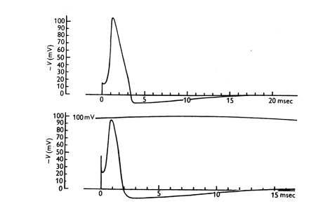
Figure 2: The above curve uses the H-H model to numerically simulate the neuronal membrane potential, taking a 15mV voltage as the initial activation voltage, calculated at 9 degrees Celsius. The following figure is the actual measured membrane potential curve. The vertical axis of the two has the same dividing value, and the horizontal axis is controlled by the scaling factor, so there are some differences. However, in general, the H-H model has a very good effect on the fitting of experimental data. This figure is derived from the origin paper5.
2.2. Integrate-And-Fire model
The Integrate-and-Fire ( IF ) model is one of the most commonly used models for analyzing nervous system behavior. In this model, the membrane potential of neurons is determined by the input current of other synapses and the injected current to the cell body. When the membrane potential reaches a threshold, an action potential ( pulse ) is generated, but the actual changes associated with the membrane voltage and the conductance driving the action potential do not form part of the model. The synaptic inputs of many neuron models derived from IF models are considered to be random, such as being described as a time-uniform Poisson process \cite{IFreview}. Because it can carry out a mathematical analysis and is complex enough to capture many basic characteristics of neural processing, IF and its derivative models are more commonly used in neural network simulation than H-H models.
The establishment of the IF model has the same physical background as the H-H model :
where
generally speaking,
Where
The IF model has made great efforts in simplifying the calculation, and also explained the working mechanism of the brain through many probability-based methods. This type of model makes it possible to use SNN to build a larger-scale neural network by finding a compromise representation in biology and computer science, rather than focusing on the simulation of a single node, which opens up a creative path for the development of SNN. However, with the rise of ANN and other classical machine learning algorithms, such models are not competitive in various tasks because they do not have appropriate training methods, especially supervised learning methods, and are difficult to use the rapidly developing computing power. Most of the research is still in the theoretical research stage.
2.3. Leaky Integrate-And-Fire model
In 1997, the pioneering spiking neuron model came out, and the concept of a third-generation neural network was really established. The basis of this model evolved from the fundamental equation of the IF model :
where u is the membrane potential,
Where
The function that determines whether the neuron outputs is the pulse activation function f, that is :
Further, if
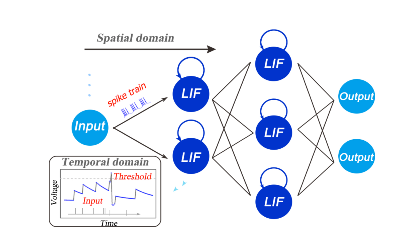
Figure 3: The data flow process of the neural network constructed by the LIF model. This diagram comes from[12](#STBP).
Through these models, LIF has developed more variants. Taking the diffusion model as an example, the author regards the change of membrane potential as a diffusion process based on the Markov process. Substituting the leakage current, the mean value of the input is
The LIF model is certainly well suited for computer modeling, but there is a fatal problem that the activation function f is not differentiable. In unsupervised learning methods such as STDP based on Hebb learning, this is not a problem, because Hebb learning methods do not involve gradient calculation. But for supervised learning, especially based on BP backpropagation algorithm, a parseable network structure is very important, so more models are proposed to solve the problem of SNN supervised learning.
2.4. Spike Response Mode
Spike Response Mode(SRM) solves the LIF model non-differentiable problem \ cite { SRM }. This model replaces the traditional LIF differential model with a function of input and output pulses. Specifically, the membrane potential of a neuron at time t can be expressed as :
The above model is divided into two parts. The first part $ \sum_f \eta(t − t(f)) $ is the sum of the pulses emitted by the neuron.
The second part is the contribution of the input current.
The constructed spiking neuron is a better differentiable model. But SRM is still more complex and not as easy to implement as LIF.
2.5. Leaky Integrate-and-Analog-Fire Model
The 0-1 coded pulse data of the LIF model is very simple and the operation mode is very suitable for training on neuromorphic processors. However, the activation mechanism of neurons behind LIF and its natural temporal information processing ability are far from being fully explored. In fact, the pulse signal of the neuron is not a simple digital signal, but an analog signal with digital signal characteristics. Its amplitude contains meaningful information as well as its frequency and emission time. However, LIF discards this information and brings about the problem of non-differentiability. Although STBP algorithm has proposed relevant solutions, it still cannot get rid of the problem of low information and low accuracy carried by SNN.
A very natural improvement idea is to simulate the pulse signal, so we propose the Leaky Integrate-and-Analog Fire ( LIAF ) model. The development of the second-generation artificial neural networks ( ANNs ) has also spawned a large number of excellent activation functions that can be used to simulate the generation of pulse signals, such as Sigmoid, RELU family activation function and so on. These functions generally have good nonlinear and resolvable characteristics, and some functions also have good data organization ability. Using these functions, a more universal SNN model can be proposed by turning the pulses between neurons into analog quantities. Specifically,
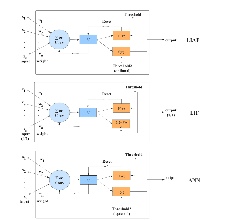
Figure 4: Comparison of three basic models: LIAF, LIF, and ANNs. LIAF and LIF naturally have the ability to process temporal information, and can also handle static information well, which is the natural inheritance form of ANNs. The difference between LIAF and LIF is only whether the synaptic transmission is an analog signal or a digital signal.
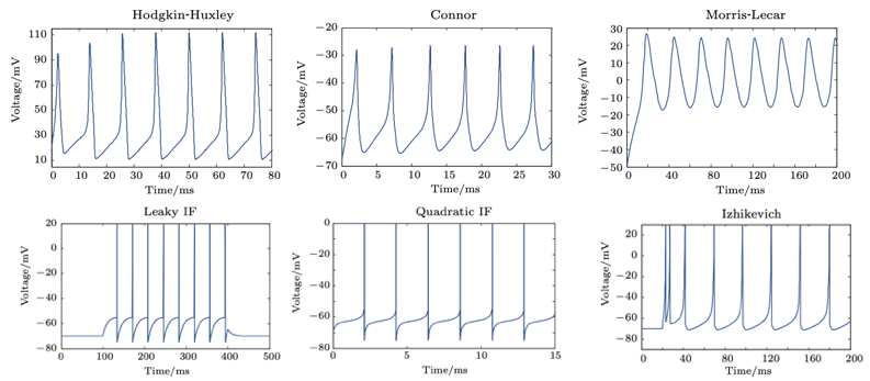
Figure 5: Different dynamics among different neural models.
3. Spike Coding Theory
3.1. Rate coding
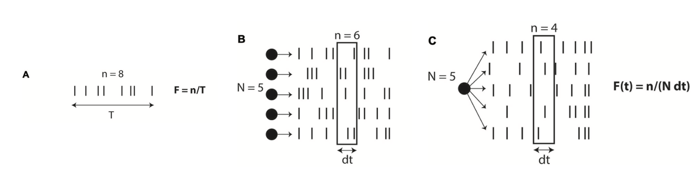
Figure 6: history
3.2. Temporal coding
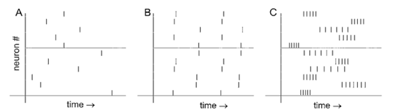
Figure 7: history
4. Training method of SNN
\label{sec:1-trainingmethod}
The training method of SNN evolves with the evolution of the model. The neurons of SNN are computational models that describe the basic laws of biological neurons, and the training algorithm of SNN is the driving force for their work. For different neuron models, different training methods and coding methods have also been developed. SNN training, like ANNs, adjusts the parameters and structure of the network through a data-oriented learning process. For SNN, different connection methods and connection weights correspond to the strength of connections between neurons, and even the presence or absence of synaptic connections. In spiking neurons, the data is often composed of a pulse sequence, which can be digital or analog. In the pulse-based learning method, SNN is trained using such temporal information, so it has obvious sparseness and efficiency advantages. Generally, the simplest representation of a pulse sequence is as follows :
Among them, $ \delta(t)$ is a Dirac function, which is 1 only at 0, and the value at other times is 0. In supervised learning, the purpose of training SNN is to make the output pulse sequence of the network as similar as possible to the target pulse sequence. Supervised learning has developed algorithms such as ReSuMe, STBP, SpikeProp, and Tempotron. At the same time, due to the rapid development of ANNs, the use of ANNs structure for training, and then mapped to the SNN, using the mechanism of SNN for reasoning, has also become a fast and effective SNN training method, called transformation-based SNN training method. In the field of unsupervised learning, based on Hebb's theory, a series of learning methods are also proposed.
4.1. Algorithm Based on Hebb Learning
In the early days, when the learning algorithm based on gradient backpropagation has not become the frontier of machine learning, most of the attempts to use simulated neural networks for learning used algorithms based on Hebb learning, including the later proposed STDP algorithm. According to Hebb learning, the strength of the relationship between the strength of the neuron connection is adjusted by continuous learning. If two associated neurons are always stimulated by associated stimuli, then the connection between the two neurons should be strengthened, and vice versa. Such a learning method is often an unsupervised process because it does not have the feedback ability in the training of label information. At the same time, such algorithms are often based on event probability, that is, the training goal is to make the correct output neuron emit more pulses randomly ( rather than have an accurate target pulse sequence ).
4.2. Algorithm Based on Gradient and Back Propagation
In unsupervised learning, the training of SNN based on STDP has achieved good results, while the method based on transformation has achieved the best performance, but the supervised learning of SNN, it has been progressing slowly. Most of the supervised learning relies on error backpropagation, and most of the work that relies on backpropagation is to estimate a differentiable approximation function for spiking neurons, thereby performing gradient descent optimization.
Tempotron algorithm is a kind of SNN supervised learning algorithm. The training target is transformed from the previous output pulse sequence into the expected output membrane potential. The basic model of this algorithm is to sum the pulse inputs of all the presynaptic spiking neurons by weighting and obtain
Here, $ \omega_i $ is the synaptic weight,
Here
The Tempotron model suggests that synaptic changes depend on the value of postsynaptic voltage. The key role of postsynaptic voltage in inducing long-term plasticity has been confirmed in some studies. The neuron model adopted by Tempotron is a trainable model, which successfully realizes the classification of single-pulse Spatio-temporal patterns, but it cannot be well extended to multi-layer network structure.
SpikeProp algorithm SpikeProp algorithm also uses the SRM model mentioned above. In order to solve the problem that neurons in the SRM model, firing pulses will bring discontinuity, it is mandatory to limit each neuron to only one pulse during each data forward propagation. SpikeProp uses a loss function that describes the similarity of pulse sequences. Taking MSE as an example, the loss function is as follows :
where m is the number of neurons,
Then there will be :
where y is the postsynaptic membrane potential,
STBP algorithm : After the rapid development of ANNs, based on BP algorithm and a large number of mature programming frameworks, accelerated hardware, and different continuous processing of data developed the STBP algorithm and pulse sequence convolution learning algorithm and so on. They all have a common idea, that is, to make SNN a continuous approximation, and then use the mature automatic gradient solution framework and optimizer for supervised learning of gradient backpropagation. The proposal of this method makes SNN have a better performance in supervised learning, the implementation difficulty is low and the versatility is good.
For the STBP algorithm, can do a perceptual understanding. At the neuron level, the neural signal will be zoned
4.3. Algorithm Based on Conversion
Although the computational efficiency is higher, the supervised learning method does not outperform the transformation-based method in terms of the accuracy of large-scale tasks. Due to the low learning accuracy of SNN, deep SNN is difficult to train. Unsolved This problem Sengupta \ cite { HSLearning } and others have proposed a way for SNN to approach ANNs using the idea of transfer learning. That is, the trained ANN network is replaced by the SNN model layer by layer. The SNN trained on this basis can have a certain performance improvement, and can also achieve a deeper SNN. Such a transformation algorithm refers to the ANNs with the same input-output mapping relationship as the SNN, through remapping and normalization, data recording ( for example, converting the original output value to the pulse rate ) into an SNN capable of processing the same data to solve the training burden of the SNN. However, in the process of transformation, there are often many factors that cause a loss of accuracy. For example, pulse rate coding does not support negative rate, and negative output often occurs in ANNs training, so it needs to be discarded. As a result, in most cases, the transformed SNN is still not comparable to the original trained ANNs, but this method still achieves the highest accuracy that large-scale spiking neural networks can achieve in image dataset classification ( including the ImageNet dataset ).
5. Discussion
Compared with ANN, SNN has more information coding methods, such as time domain coding, space-time coding, group coding, bayesian coding, time delay coding, sparse coding, etc. Therefore, SNN has great potential in dealing with complex Spatio-temporal information and multi-modal information tasks. On the other hand, the discontinuity of the SNN neuron model, the complexity of Spatio-temporal coding, and the uncertainty of network structure makes it difficult to describe the whole network mathematically and construct an effective and general learning algorithm, which limits its computational scale and accuracy.