Approximation Algorithms: Covering problems
This is the lecture notes from Chandra Chekuri's CS583 course on Approximation Algorithms. Chapter 2: Covering problems. You can read Chapter 3: Knapsack, here. Chapter 1: Introduction, here.
Chapter 2
Part of these notes were scribed by Abul Hassan Samee and Lewis Tseng.
Packing and Covering problems together capture many important problems in combinatorial optimization. We will discuss several covering problems in this chapter. Two canonical one problems are Minimum Vertex Cover and its generalization Minimum Set Cover. (Typically we will omit the use of the qualifiers minimum and maximum since this is often clear from the definition of the problem and the context.) They play an important role in the study of approximation algorithms.
A vertex cover in an undirected graph is a set of vertices such that for each edge , at least one of its end points is in . It is also called a node cover. In the Vertex Cover problem, our goal is to find a smallest vertex cover of . In the weighted version of the problem, a weight function is given, and our goal is to find a minimum weight vertex cover of . The unweighted version of the problem is also known as Cardinality Vertex Cover. Note that we are picking vertices to cover the edges. Vertex Cover is -Hard and is on the list of problems in Karp's list.
In the Set Cover problem the input is a set of elements, and a collection of subsets of such that . Our goal in the Set Cover problem is to select as few subsets as possible from such that their union covers . In the weighted version each set has a non-negative weight the goal is to find a set cover of minimim weight. Closely related to the Set Cover problem is the Maximum Coverage problem. In this problem the input is again and but we are also given an integer . The goal is to select subsets from such that their union has the maximum cardinality. Note that Set Cover is a minimization problem while Maximum Coverage is a maximization problem. Set Cover is essentially equivalent to the Hitting Set problem. In Hitting Set the input is and but the goal is to pick the smallest number of elements of that cover the given sets in . In other words we are seeking a set cover in the dual set system. It is easy to see Vertex Cover is a special case of Set Cover.
Set Cover is an important problem because in discrete optimization. In the standard definition the set system is given explicitly. In many applications the set system is implicit, and often exponential in the explicit part of the input; nevertheless such set systems are ubiquitious and one can often obtain exact or approximation algorithms. As an example consider the well known problem in graphs. One way to phrase is the following: given an edgeweighted graph find a minimum cost subset of the edges that cover all the cuts of ; by cover a cut we mean that at least one of the edges in must be chosen. This may appear to be a strange way of looking at the problem but this view is useful as we will see later. Another implicit example is the following. Suppose we are given rectangles in the plane and the goal is to choose a minimum number of points in the plane such that each input rectangle contains one of the chosen points. This is perhaps more natural to view as a special case of the Hitting Set problem. In principle the set of points that we can choose from is infinite but it can be seen that we can confine our attention to vertices in the arrangement of the given rectangles and it is easy to see that there are only vertices–however, explicity computing them may be expensive and one may want to treat the problem as an implicit one for the sake of efficiency. want to think of
Covering problems have the feature that a superset of a feasible solution is also a feasible solution. More abstractly one can cast covering problems as the following. We are given a finite ground set (vertices in a graph or sets in a set system) and a family of feasible solutions where is upward closed; by this we mean that if and then . The goal is to find the smallest cardinality set in . In the weighted case has weights and the goal is to find a minimum weight set in . In some case one can also consider more complex non-additive objectives that assign a cost for each .
2.1 Greedy for Set Cover and Maximum Coverage
In this section we consider the unweighted version of Set Cover.
2.1.1 Greedy Algorithm
A natural greedy approximation algorithm for these problems is easy to come up with.
- repeat
- A.pick the set that covers the maximum number of uncovered elements
- B.mark elements in the chosen set as covered
- until done
In case of Set Cover, the algorithm Greedy Cover is done when all the elements in set have been covered. And in case of Maximum Coverage, the algorithm is done when exactly subsets have been selected from .
We will prove the following theorem.
Theorem 2.1. Greedy Cover is a approximation for Maximum Coverage , and a approximation for Set Cover.
The following theorem due to Feige[1] implies that Greedy Cover is essentially the best possible in terms of the approximation ratio that it guarantees.
Theorem 2.2. Unless , there is no approximation for Set Cover. Unless , for any fixed , there is no approximation for Maximum Coverage.
Recently the preceding theorem has been strengthened so that the hardness holds under the assumption that [2].
2.1.2 Analysis of Greedy Cover
We proceed towards the proof of Theorem 10.3 by providing analysis of Greedy Cover separately for Set Cover and Maximum Coverage.
Analysis for Maximum Coverage
Let denote the value of an optimal solution to the Maximum Coverage problem; this is the maximum number of elements that are covered by sets in the given set system. Let denote the number of new elements covered by the -th set chosen by Greedy Cover. Also, let be the total number of elements covered after iterations, and . Note that, according to our notation, and is the number of elements chosen by Greedy Cover at the end of the algorithm, and . The key to the analysis is the following simple claim.
Claim 2.1.1. For .
Proof. Let be the elements covered by some fixed optimum solution; we have . Consider iteration . Greedy Cover selects the subset whose inclusion covers the maximum number of uncovered elements. Since is the total number of elements covered upto iteration , at least elements from are uncovered. Let the set of uncovered elements from at the end of iteration be . Since sets together cover , and hence as well, there must be some set in that collection of sets that covers at least elements. This is a candidate set that can be chosen in iteration . Since the algorithm picks the set that covers the maximum number of uncovered elements, the chosen set in iteration covers at least uncovered elements. Hence, .
Remark 2.1. It is tempting to make a stronger claim that . This is however false, and it is worthwhile to come up with an example.
By definition we have is the total number of elements covered by Greedy Cover. To analyze the worst-case we want to make this sum as small as possible given the preceding claim. Heuristically (which one can formalize), one can argue that choosing minimizes the sum. Using this one can argue that the sum is at least . We give a formal argument now.
Claim 2.1.2. For .
Proof. By induction on . The claim is trivially true for since . We assume inductively that . Then
The preceding claims yield the following lemma for algorithm Greedy Cover when applied on Maximum Coverage.
Lemma 2.1. Greedy Cover is a approximation for Maximum Coverage.
Proof. It follows from Claim 2.1.2 that . Hence, .
We note that .
Analysis for Set Cover
Let denote the value of an optimal solution to the Set Cover problem. Then an optimal solution value to the Мaximum Coverage problem with the same system and would by since it is possible to cover all the elements in set with sets. From our previous analysis, . Therefore, at most elements would remain uncovered after the first steps of Greedy Cover. Similarly, after steps of Greedy Cover, at most elements would remain uncovered. This easy intuition convinces us that Greedy Cover is a approximation for the Set Cover problem. A more formal proof is given below.
Lemma 2.2. Greedy Cover is a approximation for Set Cover.
Proof. Since , after steps,
Thus, after steps, at most elements are left to be covered. Since Greedy Cover picks at least one element in each step, it covers all the elements after picking at most sets.
A useful special case of Set Cover is when all sets are "small". Does the approximation bound for Greedy improve? We can prove the following corollary via Lemma 2.2.
Corollary 2.3. If each set in the set system has at most d elements, then Greedy Cover is a approximation for Set Cover.
Proof. If each set has at most elements then we have that and hence . Then the claim follows from Lemma 2.2.
Theorem 10.3 follows directly from Lemma 2.1 and 2.2.
A near-tight example for Greedy Cover when applied on Set Cover: Let us consider a set of elements along with a collection of subsets of . Let us also assume that and , as illustrated in Fig. 2.1.
Clearly, the optimal solution consists of only two sets, i.e., and . Hence, . However, Greedy Cover will pick each of the remaining sets, namely . Since , we get . One can construct tighter examples with more involved analysis.
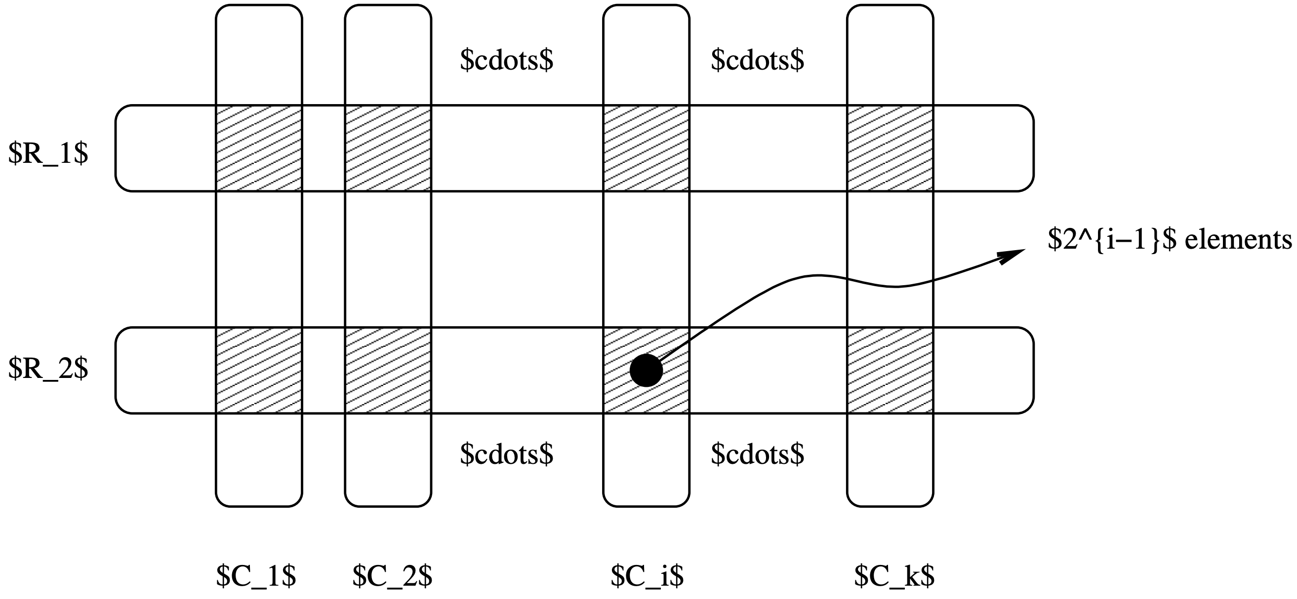
Figure 2.1: A near-tight example for Greedy Cover when applied on Set Cover
Exercise 2.1. Consider the weighted version of the Set Cover problem where a weight function is given, and we want to select a collection of subsets from such that , and is the minimum. One can generalize the greedy heuristic in the natural fashion where in each iteration the algorithm picks the set that maximizes the ratio of the number of elements to its weight. Adapt the unweighted analysis to prove that the greedy algorithm yields an approximation for the weighted version (you can be sloppy with the constant in front of .
2.1.3 Dominating Set
A dominating set in a graph is a set such that for each , either , or some neighbor of is in . In other words covers/dominates all the nodes in . In the Dominating Set problem, the input is a graph and the goal is to find a smallest sized dominating set in .
Exercise 2.2. 1. Show that Dominanting Set is a special case of Set Cover.
-
What is the greedy heuristi when applied to Dominating Set. Prove that it yields an
approximation where is the maximum degree in the graph. -
Show that Set Cover can be reduced in an approximation preserving fashion to Dominating Set. More formally, show that if Dominating Set has an
-approximation where is the number of vertices in the given instance then Set Cover has an -approximation.
2.2 Vertex Cover
We have already seen that the Vertex Cover problem is a special case of the Set Cover problem. The Greedy algorithm when specialized to Vertex Cover picks a highest degree vertex, removes it and the covered edges from the graph, and recurses in the remaining graph. It follows that the Greedy algorithm gives an approximation for the unweighted versions of the Vertex Cover problem. One can wonder whether the Greedy algorith has a better worstcase for Vertex Cover than the analysis suggests. Unfortunately the answer is negative and there are examples where the algorithm outputs a solution with vertices.
We sketch the construction. Consider a bipartite graph where is partitioned into where has vertices. Each vertex in is connected to exactly distinct vertices of ; thus, any vertex is incident to at most one edge from . It can be seen that the degree of each vertex is roughly . Clearly is a vertex cover of since the graph is bipartite. Convince yourself that the Greedy algorithm will pick all of starting with the lone vertex in (one may need to break ties to make this happen but the example can be easily perturbed to make this unnecessary). We have and and Greedy outputs a solution of size .
2.2.1 A 2-approximation for Vertex Cover
There is a very simple -approximation algorithm for the Cardinality Vertex Cover problem.
- Compute a maximal matching
in - for each edge
do - A.add both
and to - Output
Theorem 2.4. is a -approximation algorithm.
The proof of Theorem follows from two simple claims.
Claim 2.2.1. Let be the size of the vertex cover in an optimal solution. Then .
Proof. Any vertex cover must contain at least one end point of each edge in since no two edges in intersect. Hence .
Claim 2.2.2. Let . Then is a vertex cover.
Proof. If is not a vertex cover, then there must be an edge such that neither of its endpoints are in . But then can be included in , which contradicts the maximality of .
We now finish the proof of Theorem 2.4. Since is a vertex cover, Claim 2.2.1 implies that .
Weighted Vertex Cover: The matching based heuristic does not generalize in a straight forward fashion to the weighted case but -approximation algorithms for the Weighted Vertex Cover problem can be designed based on rounding.
2.2.2 Set Cover with small frequencies
Vertex Cover is an instance of Set Cover where each element in is in at most two sets (in fact, each element was in exactly two sets). This special case of the Set Cover problem admits a 2-approximation algorithm. What would be the case if every element is contained in at most three sets? More generally, given an instance of Set Cover, for each , let denote the number of sets containing . Let , which we call the maximum frequency.
Exercise 2.3. Give an -approximation for Set Cover, where is the maximum frequency of an element. Hint: Follow the approach used for Vertex Cover.
2.3 Vertex Cover via LP
Let be an undirected graph with arc weights . We can formulate Vertex Cover as an integer linear programming problem as follows. For each vertex we have a variable . We interpret the variable as follows: if if is chosen to be included in a vertex cover, otherwise . With this interprtation we can easily see that the minimum weight vertex cover can be formulated as the following integer linear program.
However, solving the preceding integer linear program is -Hard since it would solve Vertex Cover exactly. Therefore we use Linear Programming ( ) to approximate the optimal solution, , for the integer program. First, we can relax the constraint to . It can be further simplified to .
Thus, a linear programming formulation for Vertex Cover is:
We now use the following algorithm:
- Solve
to obtain an optimal fractional solution - Let
- Output
Claim 2.3.1. is a vertex cover.
Proof. Consider any edge, . By feasibility of , and thus or . Therefore, at least one of and will be in .
Claim 2.3.2. .
Proof. .
Therefore, for all instances .
Remark 2.2. For minimization problems: , where is the optimal solution found by LP; for maximization problems, .
Integrality Gap: We introduce the notion of integrality gap to show the best approximation guarantee we can obtain if we only use the values as a lower bound.
Definition 2.5. For a minimization problem , the integrality gap for a linear programming relaxation/formulation for is .
That is, the integrality gap is the worst case ratio, over all instances of , of the integral optimal value and the fractional optimal value. Note that different linear programming formulations for the same problem may have different integrality gaps.
Claims 2.3.1 and 2.3.2 show that the integrality gap of the Vertex Cover formulation above is at most .
Question: Is this bound tight for the Vertex Cover ?
Consider the following example: Take a complete graph, , with vertices, and each vertex has . It is clear that we have to choose vertices to cover all the edges. Thus, . However, for each is a feasible solution to the , which has a total weight of . So gap is , which tends to as . One can also prove that the integrality gap is essentially even in a class of sparse graphs.
Exercise 2.4. The vertex cover problem can be solved optimally in polynomial time in bipartite graphs. In fact the is integral. Prove this via the maxflowmincut theorem and the integrality of flows when capacities are integral.
Other Results on Vertex Cover
-
The current best approximation ratio for Vertex Cover is
[3]. -
There is a polynomial time approximation scheme (
), that is a approximation for any fixed , for planar graphs. This follows from a general approach due to Baker [6]. The theorem extends to more general classes of graphs.
2.4 Set Cover via LP
The input to the Set Cover problem consists of a finite set , and subsets of . Each set has a non-negative weigh and the goal is to find the minimum weight collection of sets which cover all elements in (in other words their union is ).
A linear programming relaxation for Set Cover is:
And its dual is:
We give several algorithms for Set Cover based on this primal/dual pair s.
2.4.1 Deterministic Rounding
- Solve
to obtain an optimal solution , which contains fractional numbers. - Let
- Output
Note that the above algorithm, even when specialized to Vertex Cover is different from the one we saw earlier. It includes all sets which have a strictly positive value in an optimum solution to the .
Let be an optimal solution to the primal , be an optimum solution to the dual, and let . First, note that by strong duality, . Second, by complementary slackness if then the corresponding dual constraint is tight, that is .
Claim 2.4.1. The output of the algorithm is a feasible set cover for the given instance.
Proof. Exercise.
Claim 2.4.2. .
Proof.
Notice that the the second equality is due to complementary slackness conditions (if , the corresponding dual constraint is tight), the penultimate inequality uses the definition of , and the last inequality follows from weak duality (a feasible solution for the dual problem is a lower bound on the optimal primal solution).
Therefore we have that the algorithm outputs a cover of weight at most . We note that can be as large as in which case the bound given by the algorithm is quite weak. In fact, it is not hard to construct examples that demonstrate the tightness of the analysis.
Remark 2.3. The analysis cruically uses the fact that is an optimal solution. On the other hand the algorithm for Vertex Cover is more robust and works with any feasible solution . It is easy to generalize the earlier rounding for Vertex Cover to obtain an -approximation. The point of the above rounding is to illustrate the utility of complementary slackness.
2.4.2 Randomized Rounding
Now we describe a different rounding that yields an approximation bound that does not depend on .
, and let be an optimal solution to the - for
to do - A.pick each
independently with probability - B.if
is picked, - Output the sets with indices in
Claim 2.4.3. .
Intuition: We know that . Subject to this constraint, if we want to minimize the probability that element is covered, one can see that the minimum is achieved with for each set that covers ; here is the number of sets that cover . Then the probability is .
Proof. We use the inequality for all .
We then obtain the following corollaries:
Corollary 2.6. .
Corollary 2.7. .
Proof. Via the union bound. The probability that is not covered is at most , hence the probability that there is some that is not covered is at most .
Now we bound the expected cost of the algorithm. Let cost of sets picked in iteration , then , where denotes the expectation of a random variable . Then, let ; we have . By Markov's inequality, , hence . Therefore, and all items are covered . Thus, the randomized rounding algorithm, with probability close to succeeds in giving a feasible solution of cost . Note that we can check whether the solution satisfies the desired properties (feasibility and cost) and repeat the algorithm if it does not.
-
We can check if solution after rounding satisfies the desired properties, such as all elements are covered, or cost at most
. If not, repeat rounding. Expected number of iterations to succeed is a constant. -
We can also use Chernoff bounds (large deviation bounds) to show that a single rounding succeeds with high probability (probability at least
). -
The algorithm can be derandomized. Derandomization is a technique of removing randomness or using as little randomness as possible. There are many derandomization techniques, such as the method of conditional expectation, discrepancy theory, and expander graphs.
-
After a few rounds, select the cheapest set that covers each uncovered element. This has low expected cost. This algorithm ensures feasibility but guarantees cost only in the expected sense. We will see a variant on the homework.
Randomized Rounding with Alteration: In the preceding analysis we had to worry about the probability of covering all the elements and the expected cost of the solution. Here we illustrate a simple yet powerful technique of alteration in randomized algorithms and analysis. Let be the maximum set size.
, and let be an optimal solution to the - Add to
each independently with probability , - Let
be the elements uncovered by the chosen sets in - For each uncovered element
do - A.Add to
the cheapest set that covers - Output the sets with indices in
The algorithm has two phases. A randomized phase and a fixing/altering phase. In the second phase we apply a naive algorithm that may have a high cost in the worst case but we will bound its expected cost appropriately. The algorithm deterministically guarantees that all elements will be covered, and hence we only need to focus on the expected cost of the chosen sets. Let be the random cost of the sets chosen in the first phase and let be the random cost of the sets chosen in the second phase. It is easy to see that . Let be the event that element is not covered after the first randomized phase.
Exercise 2.5. .
The worst case second phase cost can be upper bounded via the next lemma.
Lemma 2.3. Let be the cost of the cheapest set covering . Then .
Proof. Consider an element . We have the constraint that . Since each set covering has cost at least , we have . Thus,
Now we bound the expected second phase cost.
Lemma 2.4. .
Proof. We pay for a set to cover element in the second phase only if it is not covered in the first phase. Hence . Note that the events for different elements are not necessarily independent, however, we can apply linearity of expectation.
Combining the expected costs of the two phases we obtain the following theorem.
Theorem 2.8. Randomized rounding with alteration outputs a feasible solution of expected cost .
Note that the simplicity of the algorithm and tightness of the bound.
Remark 2.4. If the Set Cover problem becomes the Edge Cover problem in a graph which is the following. Given an edge-weighted graph , find the minimum weight subset of edges such that each vertex is covered. Edge Cover admits a polynomial-time algorithm via a reduction to the minimum-cost matching problem in a general graph. However for Set Cover is -Hard via a reduction from 3-D Matching.
2.4.3 Dual-fitting
In this section, we introduce the technique of dual-fitting for the analysis of approximation algorithms. At a high-level the approach is the following:
-
Consider an algorithm that one wants to analyze.
-
Construct a feasible solution to the dual
based on the structure of the algorithm. -
Show that the cost of the solution returned by the algorithm can be bounded in terms of the value of the dual solution.
Note that the algorithm itself need not be based. Here, we use Set Cover as an example. See the previous section for the primal and dual formulations for Set Cover.
We can interpret the dual as follows: Think of as how much element is willing to pay to be covered; the dual maximizes the total payment, subject to the constraint that for each set, the total payment of elements in that set is at most the cost of the set.
We rewrite the Greedy algorithm for Weighteed Set Cover.
; - While
do - A.
; - B.
; - C.
. - end while;
- Output sets in
as cover
Let be the the Harmonic number. It is well known that .
Theorem 2.9. Greedy Set Cover picks a solution of cost , where is the maximum set size, i.e., *.
To prove this, we augment the algorithm to keep track of some additional information.
- While
do - A.
- B.if
is uncovered and , set ; - C.
- D.
. - Output sets in
as cover
It is easy to see that the algorithm outputs a feasible cover.
Claim 2.4.4. .
Proof. Consider when is added to . Let be the elements that are uncovered before is added. For each the algorithm sets . Hence, . Moreover, it is easy to see that the sets are disjoint and together partition . Therefore,
For each , let .
Claim 2.4.5. is a feasible solution for the dual .
Suppose the claim is true, then the cost of Greedy Set Cover's solution = . The last step is because any feasible solution for the dual problem is a lower bound on the value of the primal (weak duality).
Now, we prove the claim. Let be an arbitrary set, and let . Let , where we the elements are ordered such that is covered by Greedy no-later than , and is covered no later than and so on.
Claim 2.4.6. For .
Proof. Let be the set that covers in Greedy. When Greedy picked the elements from were uncovered and hence Greedy could have picked as well. This implies that the density of when it was picked was no more than . Therefore which is set to the density of is at most .
From the above claim, we have
Thus, the setting of to be scaled down by a factor of gives a feasible solution.
2.4.4 Greedy for implicit instances of Set Cover
Set Cover and the Greedy heuristic are quite useful in applications because many instances are implicit, nevertheless, the algorithm and the analysis applies. That is, the universe of elements and the collection of subsets of need not be restricted to be finite or explicitly enumerated in the Set Cover problem. For instance, a problem could require covering a finite set of points in the plane using disks of unit radius. There is an infinite set of such disks, but the Greedy approximation algorithm can still be applied. For such implicit instances, the Greedy algorithm can be used if we have access to an oracle, which, at each iteration, selects a set having the optimal density. However, an oracle may not always be capable of selecting an optimal set. In some cases it may have to make the selections approximately. We call an oracle an -approximate oracle for some if, at each iteration, it selects a set such that .
Exercise 2.6. Prove that the approximation guarantee of Greedy with an approximate oracle would be for Set Cover, and for Maximum Coverage.
We will see several examples of implicit use of the greedy analysis in the course.
2.5 Submodularity
Set Cover turns out to be a special case of a more general problem called Submodular Set Cover. The Greedy algorithm and analysis applies in this more generality. Submodularity is a fundamental notion with many applications in combinatorial optimization and else where. Here we take the opportunity to provide some definitions and a few results.
Definition 2.10. Given a finite set , a real-valued set function is submodular iff
Alternatively, is a submodular function iff
The second characterization shows that submodularity is based on decreasing marginal utility property in the discrete setting. Adding element to a set will help at least as much as adding it to to a (larger) set . It is common to use to denote and to denote .
Exercise 2.7. Prove that the two characterizations of submodular functions are equivalent.
Many application of submodular functions are when is a non-negative function though there are several important applications when can be negative. A submodular function is monotone if for all and . Typically one assumes that is normalized by which we mean that ; this can always be done by shifting the function by is symmetric if for all . Submodular set functions arise in a large number of fields including combinatorial optimization, probability, and geometry. Examples include rank function of a matroid, the sizes of cutsets in a directed or undirected graph, the probability that a subset of events do not occur simultaneously, entropy of random variables, etc. In the following we show that the Set Cover and Maximum Coverage problems can be easily formulated in terms of submodular set functions.
Exercise 2.8. Let be a set and let be a finite collection of subsets of . Let , and define as: for . Show that is a monotone non-negative submodular set function.
Exercise 2.9. Let be a directed graph and let where is the number of arcs leaving . Prove that is submodular. Is the function monotone?
2.5.1 Submodular Set Cover
When formulated in terms of submodular set functions, the Set Cover problem is the following. Given a monotone submodular function (whose value would be computed by an oracle) on , find the smallest set such that . Our previous greedy approximation can be applied to this formulation as follows.
- While
do - A.find
to maximize - B.
- Output
Not so easy exercise.
Exercise 2.10.
-
Prove that the greedy algorithm is a
approximation for Submodular Set Cover? -
Prove that the greedy algorithm is a
approximation for Submodular Set Cover.
The above results were first obtained by Wolsey [7].
2.5.2 Submodular Maximum Coverage
By formulating the Maximum Coverage problem in terms of submodular functions, we seek to maximize such that . We can apply algorithm Greedy Submodular for this problem by changing the condition in line 2 to be: while .
Exercise 2.11. Prove that greedy gives a -approximation for Submodular Maximum Coverage problem when is monotone and non-negative. Hint: Generalize the main claim that we used for Мaximum Coverage.
The above and many related results were shown in the influential papers of Fisher, Nemhauser and Wolsey [8] [9].
2.6 Covering Integer Programs (CIPs)
There are several extensions of Set Cover that are interesting and useful. Submodular Set Cover is a very general problem while there are intermediate problems of interest such as Set Multicover. We refer to the reader to the relevant chapters in the two reference books. Here we refer to a general problem called Covering Integer Programs ( s for short). The goal is to solve the following integer program where is a non-negative matrix. We can assume without loss of generality that and are also non-negative.
Exercise 2.12. Prove that s are a special case of Submodular Set Cover.
One can apply the Greedy algorithm to the above problem and the standard analysis shows that the approximation ratio obtained is where (assuming that they are integers). Even though this is reasonable we would prefer a strongly polynomial bound. In fact there are instances where is exponential in and the worst-case approximation ratio can be poor. The natural relaxation of the above integer program has a large integrality gap in constrat to the case of Set Cover. One needs to strengthen the relaxation via what are known as knapsack cover inequalities. We refer the reader to the paper of Kolliopoulos and Young [10] and recent one by Chekuri and Quanrud [11] for more on this problem.
- Uriel Feige. “A threshold of ln n for approximating set cover”. In: Journal of the ACM (JACM) 45.4 (1998), pp. 634–652. ↩︎
- Dana Moshkovitz. “The Projection Games Conjecture and the NPHardness of ln
-Approximating Set-Cover”. In: Theory of Computing 11.1 (2015), pp. 221–235. ↩︎ - George Karakostas. “A better approximation ratio for the vertex cover problem”. In: ACM Transactions on Algorithms (TALG) 5.4 (2009), p. 41. ↩︎
- Irit Dinur and Samuel Safra. “On the hardness of approximating minimum vertex cover”. In: Annals of mathematics (2005), pp. 439–485. ↩︎
- Subhash Khot and Oded Regev. “Vertex cover might be hard to approximate to within 2-
”. In: Journal of Computer and System Sciences 74.3 (2008), pp. 335–349. ↩︎ - Brenda S Baker. “Approximation algorithms for NP-complete problems on planar graphs”. In: Journal of the ACM (JACM) 41.1 (1994), pp. 153–180. ↩︎
- Laurence A Wolsey. “An analysis of the greedy algorithm for the submodular set covering problem”. In: Combinatorica 2.4 (1982), pp. 385– 393. ↩︎
- Marshall L Fisher, George L Nemhauser, and Laurence A Wolsey. “An analysis of approximations for maximizing submodular set functions II”. In: Polyhedral combinatorics (1978), pp. 73–87. ↩︎
- George L Nemhauser, Laurence A Wolsey, and Marshall L Fisher. “An analysis of approximations for maximizing submodular set functions—I”. In: Mathematical Programming 14.1 (1978), pp. 265–294. ↩︎
- Stavros G Kolliopoulos and Neal E Young. “Approximation algorithms for covering/packing integer programs”. In: Journal of Computer and System Sciences 71.4 (2005), pp. 495–505. ↩︎
- Chandra Chekuri and Kent Quanrud. “On approximating (sparse) covering integer programs”. In: Proceedings of the Thirtieth Annual ACM-SIAM Symposium on Discrete Algorithms. SIAM. 2019, pp. 1596–1615. ↩︎
Recommended for you
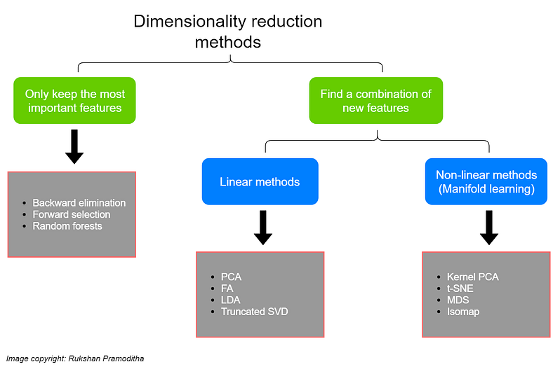
High Dimension Data Analysis - A tutorial and review for Dimensionality Reduction Techniques
This article explains and provides a comparative study of a few techniques for dimensionality reduction. It dives into the mathematical explanation of several feature selection and feature transformation techniques, while also providing the algorithmic representation and implementation of some other techniques. Lastly, it also provides a very brief review of various other works done in this space.