Spectra - High Dimension Data Analysis - A tutorial and review for Dimensionality Reduction Techniques

In the current day and age, high dimensional datasets are a common occurrence in most areas of study, with the high volume and variety of data that streams in. Research in the field of deep learning and machine learning have led to development of high efficiency models and algorithms that can deal with high volume of high dimensional datasets. However, there are techniques to engineer some significant variables and reduce the dimensionality by either eliminating other redundant variables or by creating new variables by combining a few existing ones. High dimensionality poses a few problems and hence need to be dealt with. Some of these issues are:

High number of variables lead to higher computational and time complexity of machine learning models. Reducing the dimensionality can improve the efficiency of these models.

High number of variables in a dataset, when fed to a machine learning model can lead to overfitting, thus reducing the generalizability of the machine learning models

High number of variables in a dataset may make it noisy and increases ambiguity. By reducing the dimensionality and selecting features, we can improve the information content of the dataset.

Lower dimensionality of a dataset helps in visualizing it better.

For certain models like regression models, high number of variables may include some variables which have a high correlation with the target variable. This poses the problem of multicollinearity.

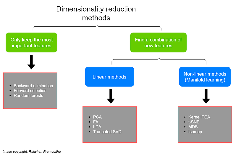
In this article, we investigate and study a few methods for selecting features from a high dimensional dataset, and thus reduce the dimensionality of the datasets.

1. Feature Selection from base features

Some techniques as described below are used to select features from the available base features in the dataset. These techniques do not alter the structure or definition of these variables, but simply select a subset of them.

1.1. Low Variance and High Correlation Filters

Statistically, variance is the measure of spread for a distribution of a random variable that determines the degree to which the values of a random variable differ from the expected value. In other words, it tells us how far the points are from the mean. The formula to variance is given by:

σ^{2} = \frac{Σ (x - \bar{x})^{2}}{n}

If the variance is closer to zero, that means the variable is fairly constant and does not spread too far away from the mean. A variable with variance 0 means all the values of the variable are constant i.e. all values are the same.

For a variable in the context of a dataset being prepared for machine learning, a variable with variance close to zero contains little to no information about the traget variable. This means it contains little impact on the target variable, and thus very little impact on the model's predictive ability.

Since variance is dependent on the range of the variable, it is important to scale the variables, especially numerical variables before computing the variance. After the variances have been computed for all the scaled variables, you can choose a threshold for the variance. All variables with variance below the theshold can be dropped.

For categorical variables, variables with few unique values but with more than 95% of the values belonging to a specific category can be dropped. For instance, if 95% of the records in a dataset belong to one particular country, say US, it is best to drop this variable as the information of the country would not improve or affect the performance of the model trained on this dataset.

Boolean features are Bernoulli random variables, and the variance of such variables is given by:

Var [X] = p (1 - p)

For Boolean variables, we would want to remove all features that are either one or zero (true or false) in more than a certain threshold. For instance, if a variable has the value 'True' for 80% of the samples or more, we drop this variable. This threshold would be achieves using the above formula

(0.8 * (1 - 0.8))

A similar feature-selection criteria can be made on the basis of the correlation of the existing features. Multiple features which are highly correlated among themeselves can lead to multicollinearity in a model. In models, especially regression models, if a feature is a linear function of 1 or more features in the dataset, it makes it difficult to estimate the relationship between each independent variable and the dependent variable independently. Thus, it is important to eliminate multicollinearity by retaining only one of the highly correlated features.

We use Pearson's correlation to find the correlation between numerical variables. To find correlations between categorical features, we can use the chi-squared test. The chi-squared statistical test considers 2 hypotheses:

H0 (Null Hypothesis) = The 2 variables to be compared are independent.

H1 (Alternate Hypothesis) = The 2 variables are dependent. Now, if the p-value obtained after conducting the test is less than 0.05, we reject the Null hypothesis and accept the Alternate hypothesis. If the p-value is greater that 0.05 we accept the Null hypothesis and reject the Alternate hypothesis i.e. it implies that the 2 variables are independent. A p-value of 0 would indicate that we can accept the alternate hypothesis with high confidence and that the two variables are highly correlated.

For determining the correlation between a categorical and a numerical variable, we can use correlation ratio (

η

) which is defined as the weighted variance of the mean of each category divided by the variance of all samples. It helps us answer a simple question: Given a continuous number, how well can you know to which category it belongs to? The score has a range of

[0, 1]

where a higher score indicates higher correlation. Using these scores, we can eliminate either of the variables in a pair that is highly correlated. One way of selecting a feature to retain, is to check the correlation of these features with the target. To train a model with good predictive ability, one should select the feature with a higher correlation with the target variable.

1.2. Recursive Feature Elimination (RFE)

Algorithm 1: Recursive Feature Elimination
$1.1$	Tune/Train the model on the training set using predictors $S_{i}, i = 1, . ., S$
$1.2$	Determine the appropriate number of features in the final model $(n)$ and the subset size (number of features to be removed in each step: $t$ )
$1.3$	While $i > n$ do:
$1.3 .1$	Calculate the importance of the predictors
$1.3 .2$	Drop lowest $t$ features on the basis of lowest importance score
$1.3 .3$	Tune/Train the model on the training set using the $S_{i - t}$ predictors
$1.3 .4$	[Optional] Calculate model performance
$1.4$	end
$1.8$	Train the model using the optimal $S_{n}$ features

Recursive Feature Elimination is wrapper-type feature selection technique. This means that a different machine learning algorithm is given and used in the core of the method, wrapped by RFE to help select features. Unlike filter-based feature selection methods that score each feature and select those features with the largest (or smallest) score, this method stops when it reaches a stopping criterion.

In RFE, we aim to select features by recursively considering smaller sets of features in each iteration. First, the estimator is trained on the initial set of features, often the entire set of predictors and the importance score of each feature is computed either through any specific attribute like feature importance, p-values, variable coefficients or a callable. Then, the least important features are pruned from current set of features, the model is re-built, and importance scores are computed again. That procedure is recursively repeated on the pruned set until the desired number of features to select is eventually reached.

One can specify the number of predictor subsets to evaluate as well as each subset’s size. Therefore, the variable subset size is a tuning parameter for RFE. The subset size that optimizes the performance criteria is used to select the predictors based on the importance rankings. The optimal subset is then used to train the final model.

One important thing to note, is that the RFE method cannot be used with all models. RFE requires that the initial model uses the full predictor set. Hence, RFE cannot be used with some models like multiple linear regression, logistic regression, and linear discriminant analysis, when the number of predictors exceeds the number of samples. To use RFE in these cases, the number of predictors must first be reduced.

1.3. Sequential Feature Selection (SFS)

Sequential Feature Selection or SFS is another wrapper-method for feature selection. SFS can be either forward or backward. You can specify the desired number of features. The feature selection algorithm removes or adds one feature at a time based on the model performance until a feature subset of the desired size

k

is reached.

Forward-SFS is a greedy algorithm that iteratively finds the best new feature to add to the set of selected features. We initially start with zero features and find the one feature that maximizes a cross-validated score when an estimator is trained on this single feature. Once that first feature is selected, we repeat the procedure by adding a new feature to the set of selected features. The procedure stops when the desired number of selected features

(k)

is reached.

Backward-SFS follows the same idea but works in the opposite direction: instead of starting with no feature and greedily adding features, we start with all the features and greedily remove features from the set. The direction parameter controls whether forward or backward SFS is used.

Algorithm 2: Backward SFS
$1.1$	Define the desired number of features
$1.2$	Tune/Train the model on the training set using all predictors
$1.3$	Compute Model Performance
$1.4$	Calculate the importance of the predictors
$1.5$	For each each subset of variables $S_{i},$ $i = 1, . . ., S$ do:
$1.5 .1$	Greedily drop the feature responsible for the worst model performance at the given point; retain $S_{i}$ predictors
$1.5 .2$	Tune/Train the model on the training set using the remaining $S_{i}$ predictors
$1.5 .3$	Calculate model performance
$1.6$	end
$1.7$	Calculate the performance profile over the final $S_{i}$ features
$1.8$	Train the model using the optimal $S_{i}$ features

While the forward SFS algorithm is easier to understand, there are minor diferences between backward SFS and RFE. SFS does not require the underlying model to expose variable coefficients or importance scores. The iterative step makes a greedy decision on the basis of the model performance. This algorithm includes a model selection on the basis of various parameters like Adj RSquared, Mallow's Cp, BIC or AIC, Accuracy or even Root Mean Squared Error (RMSE), depending on the nature of the model.

SFS may however be slower considering that more models need to be evaluated, compared to RFE. For example in backward selection, the iteration going from

m

features to

m - 1

features using k-fold cross-validation requires fitting

m * k

models, while RFE would require only a single fit.

1.3.1. Definitions of some model-selection parameters

AIC: The Akaike information criterion (AIC) is an estimator of out-of-sample prediction error and thereby relative quality of statistical models for a given set of data. It can be defined as:

A I C = - 2 \ln (L) + 2 k

Here,

k

is the number of predictors or independent features and

L

is the maximum value of the likelihood function for the model (The higher the number, the better the fit). We aim to minimize AIC, so the model with a lower AIC is selected as the better one.

BIC: Bayesian Information Criteria (BIC) is a model selection parameter defined from Bayesian probability and inference. It can be defined as:

B I C = k \ln (n) - 2 \ln (\hat{L})

Here,

(\hat{L})

is the log-likelihood of the model,

n

is the number of examples in the training dataset, and

k

is the number of parameters in the model. Like AIC, we aim to minimize the BIC too i.e. we select the model with the lowest BIC. However, unlike AIC, BIC offers a higher penalty for complex models using the sample size of the dataset. If a model is trained on a dataset with a large sample size with relatively lower number of features, the model has a lower BIC, thus making it better than a model with smaller sample size and more features.

MDL: The Minimum Description Length, or MDL for short, is a method for scoring and selecting a model. It is an information theoretic measure of model selection. It represents the minimum number of bits, or the minimum of the sum of the number of bits required to represent the data and the model and is defined as:

M D L = L (h) + L (D | h)

Here,

h

is the model,

D

is the predictions made by the model,

L (h)

is the number of bits required to represent the model, and

L (D | h)

is the number of bits required to represent the predictions from the model on the training dataset.

We also aim to reduce MDL, and hence the model with the lowest MDL is selected.

1.4. Embedded Methods: L1 regularization for Feature Selection

Let us talk about the two most common regularization techniques:

L 1

and

L 2

. These regularization terms add a penalty that can be defined as:

L1 norm penalty:

α \sum_{i = 1}^{n} | w_{i} |

L2 norm penalty:

α \sum_{i = 1}^{n} w_{i}^{2}

Here,

L 1

regularization, uses a penalty term which encourages the sum of the absolute values of the parameters to be small.

L 2

regularization, on the other hand, encourages the sum of the squares of the parameters to be small. It has frequently been observed that

L 1

regularization in many models causes many parameters to equal zero, so that the parameter vector is sparse. This makes it a natural candidate in feature selection settings, where we believe that many features should be ignored.

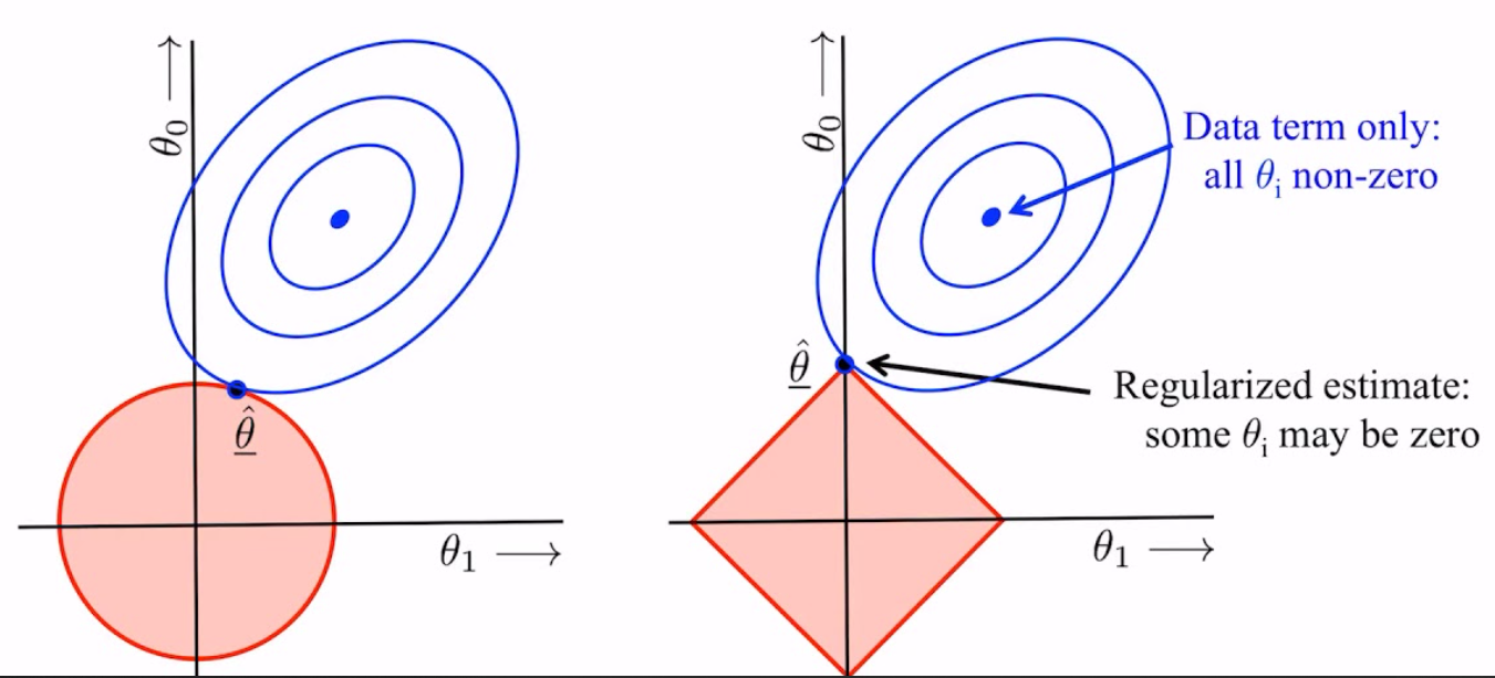Graphical representation of L2 (left) and L1 (right) regularization

In the above images, we see that

L 1

tends to generate sparser solutions than a quadratic regularizer like

L 2

. In the formula defined fo L1-norm penalty, if we increase

α

further, the solution would become sparser and sparser, i.e. more and more features would have 0 as coefficients. The orange square area in the graph above will shrink to a point corresponding to 0.

Thus, including a regularization term like L1-regularization with a machine learning model like linear regression to perform an embedded feature selection. Lasso regression uses L1 regularization on top of linear regression. It is like linear regression, but it uses a technique "shrinkage" where the coefficients of determination are shrunk towards zero.

1.5. Tree-based Feature Selection

Tree-based models can be used to compute impurity-based feature importances, which in turn can be used to discard irrelevant features. Let us consider the Random Forest models which computes importance scores for each feature based on the ‘Gini’ criterion during the training process. The Gini index is defined as follows:

Gini (D) = 1 - \sum_{i = 1}^{k} p_{i}^{2}

Here, given a dataset

D

that contains samples from

k

classes, the probability of samples belonging to class

i

at a given node can be denoted as

p_{i}

. The measure above tells us the probability of misclassifying an observation. Lower the Gini impurity, the better is the split. At every split ofa node in tree-based models, an attribute with the smallest Gini Impurity is selected for splitting the node.

In other words, a lower Gini impurity index leads to a lower likelihood of misclassification. We can use impurity-based feature importances to discard irrelevant features using a meta-transformer for selecting features based on importance weights.

2. Feature Extraction using Transformation/ Combination of Features

There are a few methods that transform existing variables in the base dataset and/or combine them with other features to reduce the dimensionality while retaining maximum information/variance in the dataset.

These methods can be classifed as linear or non-linear methods. The linear methods involve linearly projecting the original data onto a low-dimensional space and extract the transformed features. Some of these methods involve Principal Component Analysis (PCA), Factor Analysis (FA), Linear Discriminant Analysis (LDA) and Truncated Singular Value Decomposition (Truncated SVD). We will also cover some non-linear methods which work better with non-linear data.Some of those methods are: Kernel PCA, t-distributed Stochastic Neighbor Embedding (t-SNE), Multidimensional Scaling (MDS), and Isometric mapping (Isomap)

2.1. Principal Component Analysis (PCA)

In a dataset with large number of variables, it can be difficult to study and interpret the relationships between these variables. There can be too many pairwise correlations between the variables to consider. Moreover, it is difficult to visualize these variables and relationships.

To interpret the data in a more meaningful form, it is necessary to reduce the number of variables to a few, interpretable linear combinations of the data. Each linear combination will correspond to a principal component. This is the essence of PCA.

Let us assume a random vector

X

X = (\begin{matrix} X_{1} \\ X_{2} \\ ⋮ \\ X_{p} \end{matrix})

X

represents all the features, represented by each vector

X_{1}, X_{2}, . . ., X_{p}

in a dataset. If we compute the variance-covariance matrix of the vectors, it looks like:

var (X) = Σ = (\begin{array}{cccc} σ_{1}^{2} & σ_{12} & \dots & σ_{1 p} \\ σ_{21} & σ_{2}^{2} & \dots & σ_{2 p} \\ ⋮ & ⋮ & ⋱ & ⋮ \\ σ_{p 1} & σ_{p 2} & \dots & σ_{p}^{2} \end{array})

If we consider the linear combinations as below:

\begin{array}{lll} Y_{1} & = & e_{11} X_{1} + e_{12} X_{2} + \dots + e_{1 p} X_{p} \\ Y_{2} & = & e_{21} X_{1} + e_{22} X_{2} + \dots + e_{2 p} X_{p} \\ ⋮ \\ Y_{p} & = & e_{p 1} X_{1} + e_{p 2} X_{2} + \dots + e_{p p} X_{p} \end{array}

Each of the above equations represent the

Y_{i}

variables as a function of the random data

X

. Here each component

Y_{i}

represents a principal component, a combination of several features. The equations can be seen as linear regressions where you can predict

Y_{i}

from

X_{1}, X_{2}, . . . ., X_{p}

with coefficients

e_{p 1}, e_{p 2}, . . ., e_{p p}

. Since

Y_{i}

is function of the random data

X

, its variance can be represented as:

var (Y_{i}) = \sum_{k = 1}^{p} \sum_{l = 1}^{p} e_{i k} e_{i l} σ_{k l} = e_{i}^{'} Σ e_{i}

and the covariance between

Y_{i}

and

Y_{j}

can be defined as:

cov (Y_{i}, Y_{j}) = \sum_{k = 1}^{p} \sum_{l = 1}^{p} e_{i k} e_{j l} σ_{k l} = e_{i}^{'} Σ e_{j}

Now, the coefficients can be represented as a vector:

e_{i} = (\begin{matrix} e_{i 1} \\ e_{i 2} \\ ⋮ \\ e_{i p} \end{matrix})

Now, if we look at the first Principal Component:

Y_{1}

, it is the linear combination of the x-variables that has maximum variance (among all linear combinations). It accounts for as much variation in the data as possible. Hence the coefficients

e_{11,} e_{12}, \dots, e_{1 p}

are defined such that variance is maximized, given the constraint that the sum of the squared coefficients is equal to one. This constraint is required to obtain a unique answer. This means that the below variance is maximized:

var (Y_{1}) = \sum_{k = 1}^{p} \sum_{l = 1}^{p} e_{1 k} e_{1 l} σ_{k l} = e_{1}^{'} Σ e_{1}

subject to the constraint:

e_{1}^{'} e_{1} = \sum_{j = 1}^{p} e_{1 j}^{2} = 1

Similarly, the second principal component is the linear combination of x-variables that explains the maximum proportion of the remaining variation, with the constraint that the sum of the squared coefficients is equal to one and the additional constraint that the correlation between the first and second component is 0. It implies that the below variance is maximized:

var (Y_{2}) = \sum_{k = 1}^{p} \sum_{l = 1}^{p} e_{2 k} e_{2 l} σ_{k l} = e_{2}^{'} Σ e_{2}

given the first and second principal components are uncorrelated:

cov (Y_{1}, Y_{2}) = \sum_{k = 1}^{p} \sum_{l = 1}^{p} e_{1 k} e_{2 l} σ_{k l} = e_{1}^{'} Σ e_{2} = 0

All subsequent principal components have this same property – they are linear combinations that account for as much of the remaining variation as possible and they are not correlated with the other principal components. Moreover, all principal components are uncorrelated with one another.

To find coefficients

e_{i j}

for a Principal Component, we need to calculate the eigenvalues and eigenvectors of the variance-covariance matrix

Σ

. If the eigenvalues of the variance-covariance matrix are repesented by

λ_{1}, λ_{2}, . . ., λ_{p}

such that:

λ_{1} \geq λ_{2} \geq \dots \geq λ_{p}

The corresponding eigenvectors can be represented as

e_{1}, e_{2}, \dots, e_{p}

. It can be proved that the elements for these eigenvectors are the coefficients of our principal components.

Since principal components are a combination of multiple variables, interpreting it can be tough. To do so, we can look at the correlation between the principal components and the individual variables. The direction and the magnitude of the correlation score with each of the variables tells us how each principal component can be interpreted. Say a particular principal component has a strong correlation of 0.95 with a variable

X_{1}

, followed by strong correlation with 2 other variables

[X_{m}, X_{n}]

, we can say that this PC is predominantly a measure and a function of

X_{1}

. If a PC has a strong negative correlation with a variable

X_{k}

, it means the PC increases with a decreasing

X_{k}

. Thus, it is a negative function of that variable.

It is important to note that one should perform feature scaling before running PCA especially, if there is a significant difference in the scale between the features of the dataset. One can define the number of principal components to be extracted from a dataset. This could be defined using the proportion of the explained variance by each of these principal components.

2.2. Factor Analysis (FA)

Factor Analysis (FA) is a dimensionality reduction technique that also helps extract latent variables which are not directly measured in a single variable but rather inferred from other variables in the dataset. These latent variables are called factors. It models observed variables, and their covariance structure, in terms of a smaller number of these latent unobserved factors.

To understand the algorithm, let us start with a vector

X

containing all variables for all samples:

X = (\begin{matrix} X_{1} \\ X_{2} \\ ⋮ \\ X_{p} \end{matrix})

This is a random vector, with a population mean. Assume that vector of traits

X

is sampled from a population with population mean vector:

μ = (\begin{matrix} μ_{1} \\ μ_{2} \\ ⋮ \\ μ_{p} \end{matrix}) = population mean vector

Here,

E (X_{i}) = μ_{i}

denotes the population mean of variable

i

. If we consider

m

latent common factors

f_{1}, f_{2}, \dots, f_{m}

, such that

m << p

, then the common factors can be represented as :

f = (\begin{matrix} f_{1} \\ f_{2} \\ ⋮ \\ f_{m} \end{matrix}) = vector of common factors

Now, we represent each variable as a regression function of these factors as follows:

\begin{aligned} (1) & X_{1} & = μ_{1} + l_{11} f_{1} + l_{12} f_{2} + \dots + l_{1 m} f_{m} + ϵ_{1} \\ (2) & X_{2} & = μ_{2} + l_{21} f_{1} + l_{22} f_{2} + \dots + l_{2 m} f_{m} + ϵ_{2} \\ (3) & ⋮ \\ (4) & X_{p} & = μ_{p} + l_{p 1} f_{1} + l_{p 2} f_{2} + \dots + l_{p m} f_{m} + ϵ_{p} \end{aligned}

Here, the variable means

μ_{1}, . . ., μ_{p}

can be regarded as the intercepts for the multiple regression models defined above. The regression coefficients

l_{i j}

are called factor loadings and can be collected into a matrix like:

L = (\begin{array}{cccc} l_{11} & l_{12} & \dots & l_{1 m} \\ l_{21} & l_{22} & \dots & l_{2 m} \\ ⋮ & ⋮ & ⋮ \\ l_{p 1} & l_{p 2} & \dots & l_{p m} \end{array}) = matrix of factor loadings

Moreover, the error terms

(ϵ_{i})

called the specific factors. The vector for the same can be represented as:

ϵ = (\begin{matrix} ϵ_{1} \\ ϵ_{2} \\ ⋮ \\ ϵ_{p} \end{matrix}) = vector of specific factors

Each of our response variables

X

is predicted as a linear function of the unobserved common factors $f_1,f_2,...,f_m $. We have

m

unobserved factors that control the variation among our data.

The factor model has a few assumptions though:

The specific factors or random errors all have mean zero.
The common factors have variance one.
The common factors are uncorrelated with each other.
The specific factors are uncorrelated with each other.
The specific factors are uncorrelated with the common factors.

We can interpret factor analysis as an inversion of principal components analysis. While PCA represents new components as a function of combination of observed variables, FA models the observed variables as linear functions of the new unobserved variables called factors. However, both PCA and FA reduce the dimension of the dataset.

2.3. Linear Discriminant Analysis

Linear Discriminant Analysis, or LDA, is a linear machine learning algorithm used for multi-class classification. It can also be used for dimensionality reduction.

Let us assume a dataset with

K

classes (for the target variable). LDA helps us reduce the number of features to

K - 1

classes.

The aim of LDA is to:

Minimize the Inter-Class Variability: This can be done by including as many similar points within a particular class. This will ensure less number of misclassifications.

Maximize the Distance Between the Mean of Classes: It tries to keep the class means apart from each other and as far as possible. This increases the confidence during prediction.

Thus, LDA tries to separate (or discriminate) the samples in the training dataset by their class value. In this pursuit of dimensionality reduction, the model tries to find a linear combination of input variables that achieves the maximum separation for samples between classes (class centroids or means) and the minimum separation of samples within each class.

To explain this better, let us compare LDA to PCA. PCA is an unsupervised machine learning method, that is it takes into account only the spectral data and its variance to reduce the number of features. It does not require the labels of the data samples.

However, LDA makes use of the class labels to produce a dimensionality reduction that maximizes the distance between the classes. In other words, while PCA will find the projections that maximise the variance of the data irrespective of their classes, LDA will seek to maximise the distance between those classes while reducing the number of features.

In the above image, we see how LDA projects the existing features onto an exis such that it separates the two classes in the projected space. The general overview of this algorithm looks like the following:

Algorithm 3: Linear Discriminant Analysis
$1.1$	Compute the d-dimensional mean vector for the different classes from the dataset.
$1.2$	Compute the Scatter matrix (in between class and within the class scatter matrix)
$1.3$	Sort the Eigen Vector by decreasing Eigen Value and choosing $k$ eigenvector with the largest eigenvalue to from a $d \times k$ dimensional matrix $w$ (where every column represent an eigenvector)
$1.4$	Used $d \times k$ eigenvector matrix to transform the sample onto the new subspace.

Although it looks like LDA can perform better than PCA in multi-class classification models, it is not always the case. The choice depends on the performance of the model built on the transformed dataset. One can also combine LDA and PCA as an ensemble to obtain transformed features.

2.4. Truncated Singular Value Decomposition (SVD)

The Singular-Value Decomposition, or SVD, is a matrix decomposition method for reducing a matrix to its constituent parts in order to make certain subsequent matrix calculations simpler. To understand Truncated SVD, let us briefly explain SVD.

SVD is a method for low-dimensional representation of a high-dimensional matrix. In this process, it also makes it easy to eliminate the less important parts of that representation to produce an approximate representation with any desired number of dimensions. Thus, it is a dimensionality reduction technique.

Let

M

be an

m \times n

matrix and rank

r

. Now, we find matrices

U

Σ

, and

V

as shown in the image below:

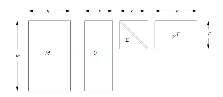Form of a singular-value decomposition

It can be mathematically represented as:

A_{m \times n} = U_{m \times m} . Σ_{m \times n} . V_{n \times n}^{T}

Let us define the above matrices:

$U$ is an $m \times r$ column-orthonormal matrix ; i.e., each of its columns is a unit vector and the dot product of any two columns is 0.
$V$ is an $n \times r$ column-orthonormal matrix. Note that we always use V in its transposed form, so it is the rows of $V^{T}$ that are orthonormal.
$Σ$ is a diagonal matrix; that is, all elements not on the main diagonal are 0. The elements of $Σ$ are called the singular values of $M$ .

The key to understanding what SVD offers is in viewing the

r

columns of

U

Σ

, and

V

as representing concepts that are hidden in the original matrix

M

. To understand how it helps in dimensionality reduction, let us suppose we want to represent a very large matrix

M

by its SVD components

U

Σ

, and

V

. However, these matrices are also too large to store conveniently. We can reduce the dimensionality of the three matrices by setting the smallest of the singular values to zero. If we set the

s

smallest singular values to 0, then we can also eliminate the corresponding

s

columns of

U

and

V

. We make the choice of setting the lowest singular values to zero when we reduce the number of dimensions minimizes the root-mean-square error (RMSE) between the original matrix

M

and its approximation.

In order to determine how many singular values need to be retained, it is a thumb-rule to retain enough singular values to make up 90% of the energy in

Σ

. This means, the sum of the squares of the retained singular values should be at least 90% of the sum of the squares of all the singular values.

In truncated SVD, we take the

k

largest singular values (such that

0 < k < r

) and their corresponding left and right singular vectors

A_{m \times n} \approx U_{t (m \times k)}, Σ_{t (k \times k)}, V_{t (k \times n)}^{T}

Contrary to PCA, this estimator does not center the data before computing the singular value decomposition. This means it can work with sparse matrices efficiently. Thus, we can used Truncated SVD as a dimensionality reduction technique for sparse datasets.

2.5. Kernel PCA

All the above methods are linear methods of dimensionality reduction. They work best for linear data. To be able to reduce the dimensions of non-linear data, we need non-linear methods. The first one discussed here is Kernel PCA. It is a non-linear version of PCA that uses kernels.

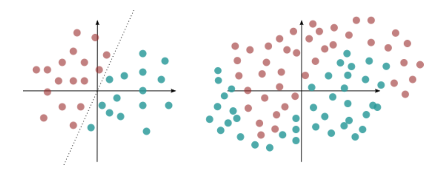Linear and Non-linear dataset

In the above figure, the data on the left is linearly separable. The one on the right is non-linear and needs a higher order polynomial to divide the complex boundary.

In the conventional PCA algorithm, the process of matrix decomposition into eigenvectors is a linear transformation. Kernel PCA can be used to reduce the dimensions of data during classification of data whose decision boundaries are described by non-linear function. The idea is to go to a higher dimension space in which the decision boundary becomes linear. Let's say the decision boundary of the above data distribution is defined by a third order polynomial

y = a + b x + c x^{2} + d x^{3}

. If we plot this function on an

x - y

plane, it will produce a wavy line, which could act as the decision boundary in the image above. Now if we project this to a higher-dimension space with axes

x, x^{2}, x^{3}

and

y

. In this 4D space, the third order polynomial becomes a linear function and the decision boundary converts into a hyperplane. So, if we find a suitable transformation to convert our data into linear data, we can proceed to the usual PCA decomposition on the transformed data.

Thus the algorithm can be simplified as below:

Algorithm 4: Kernel PCA
$1.1$	Define the original set of $n$ features as $x$
$1.2$	Define $ϕ (x)$ as the non-linear combination (mapping) of these variables into a $m > n$ dataset
$1.3$	Define the kernel function: compute the kernel function $κ (x) = ϕ (x) ϕ^{T} (x)$
$1.4$	Calculate the squared Euclidean distance between each pair of points in the dataset.
$1.5$	Pass the distance matrix through the defined kernel to compute the kernel matrix for the given dataset.
$1.6$	Calculate the eigenvalues and eigenvectors of the kernel matrix
$1.7$	Flip eigenvectors' sign to enforce deterministic output
$1.8$	Concatenate the eigenvectors corresponding to the highest $n$ (where $n$ is the number of desired components) eigenvalues.

One caveat in using Kernel PCA is that one has to define a value for the

(g a m m a)

hyperparameter, which is the kernel coefficient, before running the algorithm. One thus needs to run a hyperparameter tuning technique like Grid Search to determine an optimal value for this parameter.

2.6. t-distributed Stochastic Neighbor Embedding (t-SNE)

This is a widely used dimensionality reduction technique for data visualization, image processing and NLP. The algorithm can be described using these broad steps:

Algorithm 5: t-SNE
$1.1$	Compute the Euclidean distance matrix for all points from each other
$1.2$	Transform the distances into conditional probabilities that represent the similarity between every two points
$1.3$	Using the conditional probabilities, compute joint probability function: $p_{i j} = (p_{j \| i} + p_{i \| j}) / 2 n$ using a Gaussian function
$1.4$	Build a random dataset of points with the same number of points as in the original dataset, and $K$ features, where $K$ is the desired number of features.
$1.5$	For this new dataset, create their joint probability distribution using the t-distribution (instead of Gaussian distribution)
$1.4$	Ese the Kullback-Leiber (KL) divergence to make the joint probability distribution of the data points in the low dimension (new random dataset) as similar as possible to the one from the original dataset.
$1.5$	The new transformation gives us a new dataset with reduced dimensions

We choose t-distribution instead of the Gaussian distribution because of the heavy tails property of the t-distribution. This leads to moderate distances between points in the high-dimensional space to become extreme in the low-dimensional space, and that helps prevent “crowding” of the points in the lower dimension.

We use KL-divergence as a measure of how much two distributions are different from one another. Lower the value of KL-divergence, more similar are the distributions. To find the new dataset with the reduced dimensions, we use the gradient descent optimization. The cost function that the gradient descent tries to minimize is the KL divergence of the joint probability distribution from the high-dimensional space and the low-dimensional space.

Another advantage of using t-distribution is that it helps improve the efficiency of the gradient-descent optimization process.

2.7. Multidimensional Scaling (MDS)

MDS is a non-linear dimensionality reduction technique that tries to preserve the distances between samples while reducing the dimensionality of non-linear data. It is also known as Principal Coordinates Analysis (PCoA), Torgerson Scaling or Torgerson–Gower scaling.

The main objective of MDS is to represent dissimilarities between data points as distances between points in a low dimensional space such that the distances correspond as closely as possible to the dissimilarities. The classical MDS algorithm, also called metric scaling can be described as below:

Algorithm 6: Classical MDS
$1.1$	Given a matrix $D$ with dimesnionality $m$ , find matrix $X$ with the reduced dimension $p$
$1.2$	From matrix $D$ , compute a matrix $B$ , by applying a centering matrix to $D$
$1.3$	Determine the largest eigenvalues $(λ_{1}, λ_{2}, . . ., λ_{n - 1})$ and corresponding eigenvectors $(v_{1}, v_{2}, . ., v_{n - 1})$ of matrix $B$ w.r.t $p$
$1.4$	Get the square root of the dot product of the matrix of eigenvectors and the diagonal matrix of eigenvalues of $B$

This algorithm is now synonymous with Principal Coordinates Analysis. This is the metric MDS that deals with numerical distances, in which there is no measurement error (you have exactly one distance measure for each pair of items).

Non-metric MDS deals with non-numerical distances between items, in which there is no measurement error (you have exactly one distance measure for each pair of items). Thus, in non-metric Multidimensional Scaling, we compute a dissimilarity matrix instead of a distance matrix.

2.8. Isometric mapping (Isomap)

This non-linear technique of dimensionality reduction is an extension of MDS or Kernel PCA. This algorithms uses curved or geodesic distance to connect eah instance to its nearest neighbors and reduces dimensionality.

The broad steps of this algorithm can be described as below:

Algorithm 7: Isomap
$1.1$	Define $k$ as the arbitrary number of neighbors to be discovered for each data point
$1.2$	Use KNN-approach to find the $k$ nearest neighbors of every data point
$1.3$	Construct the neighborhood graph where points are connected to each other if they are each other’s neighbors
$1.4$	Compute the shortest path or the geodesic distance between each pair of data points using either Floyd-Warshall or Dijkstra’s algorithm
$1.5$	Use MDS to compute lower-dimensional embedding

Use of MDS ensures that each object into the N-dimensional space (where

N

is a user-defined hyperparameter) such that the between-point distances are preserved as well as possible.

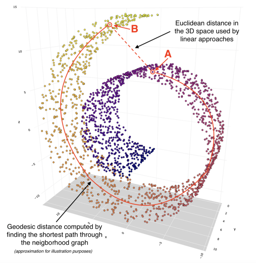Comparison of linear Euclidean distance and Geodesic distance between two points on a non-linear data representation

The use of the geodesic distance ensures that we do not misrepresent the distance between two points in a non-linear data distribution. IN the above image, if we look at points A and B, they appear to be much closer to each other if Euclidean distance is used to compute the distance between the two points. However, geodesic distances traces the path between the 2 points on the basis of the data distribution and is hence a more accurate representation of the distance between them. Use of a linear dimensionality reduction technique would hence, not be accurate.

3. AutoEncoder for Dimensionality Reduction

Autoencoders are artificial neural networks used for unsupervised learning. They are responsible for efficient coding or representation of data.

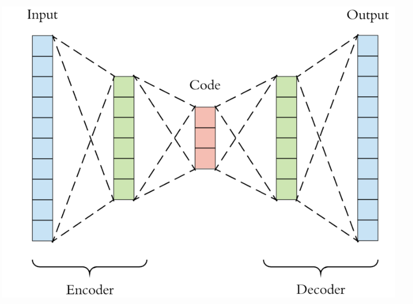Architecture of a simple autoencoder

The above image shows the architecture of a simple autoencoder. It consists of an encoder-decoder network. Here, the encoder takes the input and transforms it into a compressed representation i.e. encoding, and then passes it to the decoder. The decoder, as the name suggests, seeks to reconstruct the original representation from the encoded data, as accurately as possible. The goal is to learn an encoded representation for a dataset. Looking at the image above, it follows a bottle-neck architecture, which indicates that the dimensions of the encoded output from the encoder i smaller than the original input.

This architecture forces the autoencoder to compress the training data’s informational content, and embed it into a low-dimensional space.

Like any other neural network, there is a lot of flexibility in how autoencoders can be constructed such as the number of hidden layers and the number of nodes in each, along with the activation function of eavh layer. With each hidden layer the network will attempt to find new structures in the data.

Comparison of PCA and Autoencoder for dimensionality reduction
Parameter	PCA	Autoencoders (AE)
Data transformation	PCA follows linear transformation of data	Autoencoders can be either linear or non-linear on the basis of the activation function
Computational Efficiency	PCA is relatively faster	Autoencoders use Gradient descent optimization and is slower
Data Sample Size	PCA works best with smaller datasets	Autoencoders can be used for large datasets
Hyperparameter Tuning/ Input parameters	PCA need a hyperparameter $k$ to define number of desired features	Autoencoders have a complex architecture that needs to defined. This needs an activation function, number of dimensions in the encoding, number of nodes in each layer and number of layers in the network etc.

Let us try to construct a simple Autoencoder for dimensionality reduction:

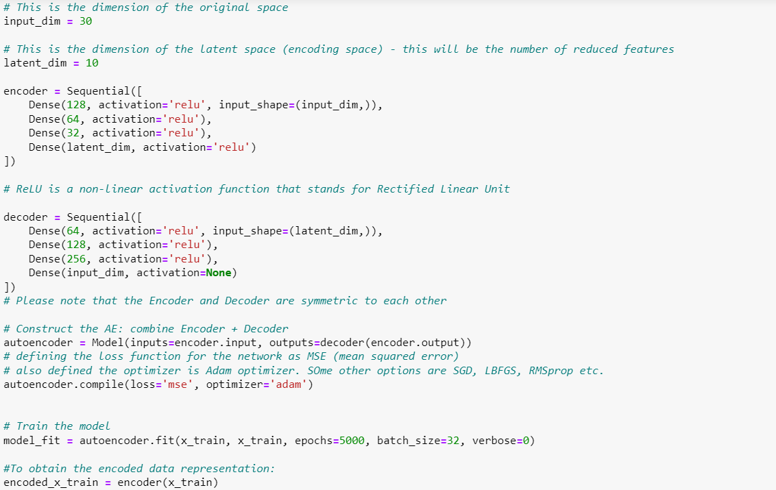Simple autoencoder for dimensionality reduction from 30 inout features to 10 features

The above autoencoder (built using Keras in Python) seeks to represent an input dataset with 30 features as an encoded space with 10 features. The encoder and decoder and constructed separately (in most cases, the AE is symmetrical i.e. the encoder and decoder are complementary to each other). At the end, they are stitched together to create the AE. We then need to train the autoencoder i.e. fit it on our dataset. We can then extract the encoded space from the encoder step of the AE.

4. Additional Algorithms for Dimensionality Reduction

4.1. LCEM: Linear dimensionality reduction algorithm based on conditional entropy minimization.

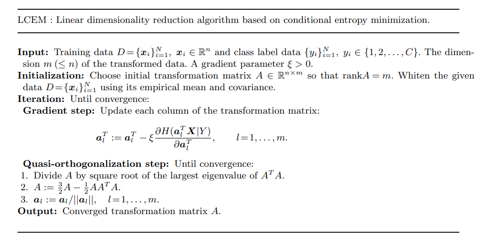LCEM algorithm

Information Theory is a branch of computer science and mathematics that deals with transmission, storage and quantification of information bits. It is also widely used in the field of machine learning to design and optimize algorithms.

In 2010, Hino and Murata proposed a dimensionality reduction based on class conditional entropy minimization. To look at dimensionality reduction from an information theoretic method, let us define the Shannon Entropy of a random variable

X

as follows:

H (X) = - \int p (x) \log p (x) d x

Here,

p

is the probability density function of

X

. Now, let us suppose this variable corresponds to data samples in a dataset which also has a class variable (dependent variable) defined by

Y

. Given

A

is a transformation matrix applied on

A

, then the class-conditonal entropy is given by:

H (A^{T} X ∣ Y) = \sum_{y = 1}^{C} \frac{N_{y}}{N} H (A^{T} X ∣ Y = y)

Here,

N_{y}

is the number of data points in a given class

y

and

N = Σ_{y = 1}^{C} N_{y}

where

y_{i} \in [1, 2, . . ., C]

is the total number of data points in the dataset. The above formula defines the class conditional entropy of a transformed random variable

A^{T} X

. In simple terms, conditional entropy represents how much uncertainty a random variable has remaining if we have already learned the value of a second random variable. This can also be interpreted as the amount of information needed to describe the outcome of a random variable given that the value of another random variable is known. Class conditional entropy, as described above, would imply the amount of uncertainty in the transformed variable $A^{T} X$ , given the information in the class variable $Y$ . In this case, since we want to find a transformation that mimics the actual information in $X$ as accurately as possible, without the loss of any information contained, we would want to reduce the uncertainty, and hence minimize the class conditional entropy.

The method described in this section, constructs a transformation

f : x \mapsto z

which minimizes the class conditional entropy

H (Z | Y)

. Now,

H (Z | Y)

will be minimized by any functions which map all data

x

to a single point. We also need to prevent overfitting by avoiding a high representational power of the transformation

f

. To avoid overfitting in the optimization of

H (Z | Y)

, we add a regularization term

ε Ψ (f, D)

which depends on both the function

f

and the given data

D

min_{f : x \mapsto z} H (Z ∣ Y) + ε Ψ (f, D) .

The above function represents the regularized conditional entropy minimization objective.

The minimization of the class conditional entropy will be done using gradient descent optimization. This means that we calculate the gradient vector of the class conditional entropies of the transformed data

z_{l} = a_{l}^{T} x, l = 1, . . ., m

and update each column of the transformation matrix

A

Since the objective is to minimize the sum of the marginal entropies, a simple optimization for each marginal entropy may lead us to the same single transformation vector

a_{l} = a, (l = 1, . . ., m)

for all the marginal entropies. To avoid this, the authors suggest quasi-orthogonalization to the transformation matrix in each iteration of gradient descent. This is defined in a three-step process as follows:

Step 1: Divide

A

by square root of the largest eigenvalue of

A^{T} A

Step 2:

A \leftarrow \frac{3}{2} A - \frac{1}{2} A A^{T} A

Step 3: Normalize the norm of each column of

A

to 1.

This optimization process is repeated until the model converges. The result at the end of this process is a converged transformation matrix

A

. As seen in the figure above, in the gradient step, a marginalized entropy is minimized by gradient descent method for each column of the transformation matrix

A

, and in the quasi-orthogonalization step, columns of

A

are quasi-orthogonalized. Thus, this algorithm above uses a linear transformation

A^{T} : x \mapsto z

to decrease the class conditional entropy while reducing the dimensions of the dataset

x

The same paper as above, also proposes another method of dimensionality reduction: MCEM or Multiple kernel learning algorithm based on conditional entropy minimization.

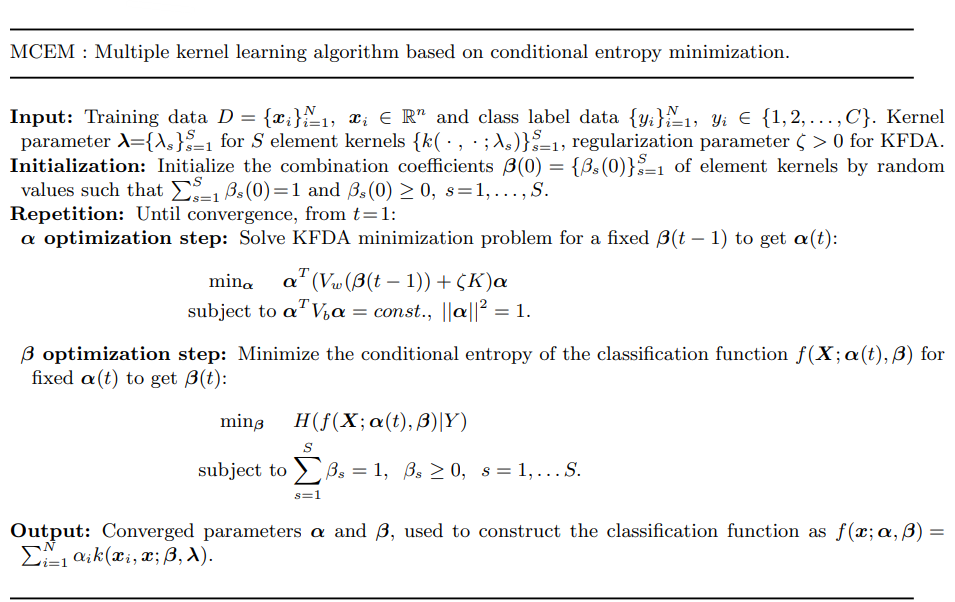
The MCEM algorithm is represented in teh image above. THe above technique extends dimensionality reduction using class conditional entropy to non-linear data. It suggests that we combine multiple kernel functions with a coefficient vector

β

, and optimize this coefficient

β

along with the weight

α

of the classification function by minimizing the conditional entropy. The detailed explanation of this method can be read in the work published by Hino et al.

5. Conclusion

This review only studies a few techniques for dimensionality reduction. There are several other techiques that have been studied in the past. In 2014, Plan et al. studied Dimension Reduction by random hyperplane tessellations. In 2012, Lee et al. published his work and review of graph-based dimension reduction techniques. Neighbourhood components analysis, suggested by Goldberger et al. in 2004 uses Mahalanobis distance measure for dimensionality reduction.

6. References

Hino, Hideitsu & Murata, Noboru. (2010). A Conditional Entropy Minimization Criterion for Dimensionality Reduction and Multiple Kernel Learning. Neural computation. 22. 2887-923. 10.1162/NECO_a_00027.
Plan, Yaniv & Vershynin, Roman. (2011). Dimension Reduction by Random Hyperplane Tessellations. Discrete and Computational Geometry. 51. 10.1007/s00454-013-9561-6
Lee, John A. & Verleysen, Michel (2012). Graph-based dimensionality reduction (https://perso.uclouvain.be/michel.verleysen/papers/bookLezoray12jl.pdf)
Goldberger, Jacob & Roweis, Sam & Hinton, Geoffrey & Salakhutdinov, Ruslan. (2004). Neighbourhood Components Analysis.. in Advances in Neural Information Processing Systems (NIPS 2004) Vancouver Canada: Dec.. 17.
Principal Component Analysis (https://online.stat.psu.edu/stat505/lesson/11)
Factor Analysis (https://online.stat.psu.edu/stat505/lesson/12)

High Dimension Data Analysis - A tutorial and review for Dimensionality Reduction Techniques

1. Feature Selection from base features

1.1. Low Variance and High Correlation Filters

1.2. Recursive Feature Elimination (RFE)

1.3. Sequential Feature Selection (SFS)

1.3.1. Definitions of some model-selection parameters

1.4. Embedded Methods: L1 regularization for Feature Selection

1.5. Tree-based Feature Selection

2. Feature Extraction using Transformation/ Combination of Features

2.1. Principal Component Analysis (PCA)

2.2. Factor Analysis (FA)

2.3. Linear Discriminant Analysis

2.4. Truncated Singular Value Decomposition (SVD)

2.5. Kernel PCA

2.6. t-distributed Stochastic Neighbor Embedding (t-SNE)

2.7. Multidimensional Scaling (MDS)

2.8. Isometric mapping (Isomap)

3. AutoEncoder for Dimensionality Reduction

4. Additional Algorithms for Dimensionality Reduction

4.1. LCEM: Linear dimensionality reduction algorithm based on conditional entropy minimization.

5. Conclusion

6. References

Recommended for you

Report Article