You can read the notes from the previous lecture of Chandra Chekuri's course on \ell_0 Sampling, and Priority Sampling here.
Suppose we have a stream a_(1),a_(2),dots,a_(n)a_{1}, a_{2}, \ldots, a_{n} of objects from an ordered universe. For simplicity we will assume that they are real numbers and more over that they are distinct (for simplicity). We would like to find the kk'th ranked element for some 1 <= k <= n1 \leq k \leq n. In particular we may be interested in the median element. We will discuss exact and approximate versions of these problems. Another terminology for finding rank kk elements is quantiles. Given a number phi\phi where 0 < phi <= 10<\phi \leq 1 we would like to return an element of rank phi n\phi n. This normalization allows us to talk about epsilon\epsilon-approximate quantiles for epsilon in[0,1)\epsilon \in[0,1). An epsilon\epsilon-approximate quantile is an element whose rank is at least (phi-epsilon)n(\phi-\epsilon) n and at most (phi+epsilon)n(\phi+\epsilon) n. In other words we are allowing an additive error of epsilon n\epsilon n. There is a large amount of literature on quantiles and quantile queries. In fact one of the earliest "streaming" papers is the one by Munro and Paterson [5] who described a pp-pass algorithm for selection using tilde(O)(n^(1//p))\tilde{O}\left(n^{1 / p}\right) space for any p >= 2p \geq 2. They also considered the "random-order" streaming setting which has become quite popular in recent years.
The material for these lectures is taken mainly from the excellent chapter/survey by Greenwald and Khanna [1]. We mainly refer to that chapter and describe here the outline of what we covered in lectures. We will omit proofs or give sketchy arguments and refer the reader to [1].
1. Approximate Quantiles and Summaries
Suppose we want to be able to answer epsilon\epsilon-approximate quantile queries over an ordered set SS of nn elements. It is easy to see that we can simply pick elements of rank i|S|//ki|S| / k for 1 <= i <= k≃1//epsilon1 \leq i \leq k \simeq 1 / \epsilon and store them as a summary and use the summary to answer any quantile query with an epsilon n\epsilon n additive error. However, to obtain these elements we first need to do selection which we can do in the offline setting if all we want is a concise summary. The question we will address is to find a summary in the streaming setting. In the sequel we will count space usage in terms of "words". Thus, the space usage for the preceding offline summary is Theta(1//epsilon)\Theta(1 / \epsilon).
We will see two algorithms. The first will create an epsilon\epsilon-approximate summary [4][4] with space O((1)/(epsilon)log^(2)(epsilon n))O\left(\frac{1}{\epsilon} \log ^{2}(\epsilon n)\right) and is inspired by the ideas from the work of Munro and Paterson. Greenwald and Khanna [2] gave a different summary that uses O((1)/(epsilon)log(epsilon n))O\left(\frac{1}{\epsilon} \log (\epsilon n)\right) space.
Following [1][1] we will think of a quantile summary QQ as storing a set of elements {q_(1),q_(2),dots,q_(ℓ)}\{q_{1}, q_{2}, \ldots, q_{\ell}\} from SS along with an interval [rmin_(Q)(q_(i)),rmax_(Q)(q_(i))][\mathbf{rmin}_{Q}(q_{i}), \mathbf{rmax}_{Q}(q_{i})] for each q_(i);rmin_(Q)(q_(i))q_{i} ; \mathbf{rmin}_{Q}(q_{i}) is a lower bound on the rank of q_(i)q_{i} in SS and rmax_(Q)(q_(i))\mathbf{rmax}_{Q}(q_{i}) is an upper bound on the rank of q_(i)q_{i} in SS. It is convenient to assume that q_(1) < q_(2) < dots < q_(ℓ)q_{1}<q_{2}<\ldots<q_{\ell} and moreover that q_(1)q_{1} is the minimum element in SS and that q_(ℓ)q_{\ell} is the maximum element in SS. For ease of notation we will simply use QQ to refer to the quantile summary and also the (ordered) set {q_(1),q_(2),dots,q_(ℓ)}\{q_{1}, q_{2}, \ldots, q_{\ell}\}.
Our first question is to ask whether a quantile summary QQ can be used to give epsilon\epsilon-approximate quantile queries. The following is intuitive and is worthwhile proving for oneself.
Lemma 1SupposeQQis a quantile summary forSSsuch that for1 <= i < ℓ,rmax_(Q)(q_(i+1))-1 \leq i<\ell, \mathbf{rmax}_{Q}\left(q_{i+1}\right)-rmin_(Q)(q_(i)) <= 2epsilon|S|\mathbf{rmin}_{Q}\left(q_{i}\right) \leq 2 \epsilon|S|. ThenQQcan be used forepsilon\epsilon-approximate quantile queries overSS.
In the following, when we say that QQ is an epsilon\epsilon-approximate quantile summary we will implicitly be using the condition in the preceding lemma.
Given a quantile summary Q^(')Q^{\prime} for a multiset S^(')S^{\prime} and a quantile summary Q^('')Q^{\prime \prime} for a multiset S^('')S^{\prime \prime} we would like to combine Q^(')Q^{\prime} and Q^('')Q^{\prime \prime} into a quantile summary QQ for S=S^(')uuS^('')S=S^{\prime} \cup S^{\prime \prime}; by union here we view SS as a multiset. Of course we would like to keep the approximation of the resulting summary similar to those of Q^(')Q^{\prime} and Q^('')Q^{\prime \prime}. Here a lemma which shows that indeed we can easily combine.
We will not prove the correctness but describe how the intervals are constructed for QQ from those for Q^(')Q^{\prime} and Q^('')Q^{\prime \prime}. Suppose Q^(')={x_(1),x_(2),dots,x_(a)}Q^{\prime}=\{x_{1}, x_{2}, \ldots, x_{a}\} and Q^('')={y_(1),y_(2),dots,y_(b)}Q^{\prime \prime}=\{y_{1}, y_{2}, \ldots, y_{b}\}. Let Q=Q^(')uuQ^('')={z_(1),z_(2),dots,z_(a+b)}Q=Q^{\prime} \cup Q^{\prime \prime}=\{z_{1}, z_{2}, \ldots, z_{a+b}\}. Consider some z_(i)in Qz_{i} \in Q and suppose z_(i)=x_(r)z_{i}=x_{r} for some 1 <= r <= a1 \leq r \leq a. Let y_(s)y_{s} be the largest element of Q^('')Q^{\prime \prime} smaller than x_(r)x_{r} and y_(t)y_{t} be the smallest element of Q^('')Q^{\prime \prime} larger than x_(r)x_{r}. We will ignore the cases where one or both of y_(s),y_(t)y_{s}, y_{t} are not defined. We set
We will refer to the above operation as COMBINE(Q^('),Q^(''))\operatorname{COMBINE}(Q^{\prime}, Q^{\prime \prime}). The following is easy to see.
Lemma 3LetQ_(1),dots,Q_(h)Q_{1}, \ldots, Q_{h} be epsilon\epsilon-approximate quantile summaries forS_(1),S_(2),dots,S_(h)S_{1}, S_{2}, \ldots, S_{h}respectively. ThenQ_(1),Q_(2),dots,Q_(h)Q_{1}, Q_{2}, \ldots, Q_{h}can be combined in any arbitrary order to obtain anepsilon\epsilon-approximate quantile summaryQ=Q_(1)uu dots uuQ_(h)Q=Q_{1} \cup \ldots \cup Q_{h}forS_(1)uu dots uuS_(h)S_{1} \cup \ldots \cup S_{h}.
Next we discuss the PRUNE(Q,k)\operatorname{PRUNE}(Q, k) operation on a quantile summary QQ that reduces the size of QQ to k+1k+1 while losing a bit in the approximation quality.
Lemma 4LetQ^(')Q^{\prime}be anepsilon\epsilon-approximate quantile summary forSS. Given an integer parameterkkthere is a quantile summaryQ subeQ^(')Q \subseteq Q^{\prime}forSSsuch that|Q| <= k+1|Q| \leq k+1and it is(epsilon+(1)/(2k))(\epsilon+\frac{1}{2 k})-approximate.
We sketch the proof. We simply query Q^(')Q^{\prime} for ranks 1,|S|//k,2|S|//k,dots,|S|1,|S| / k, 2|S| / k, \ldots,|S| and choose these elements to be in QQ. We retain their rmin\mathbf{rmin} and rmax\mathbf{rmax} values from Q^(')Q^{\prime}.
1.1. An O((1)/(epsilon)log^(2)(epsilon n):}O\left(\frac{1}{\epsilon} \log ^{2}(\epsilon n)\right. space algorithm
The idea is inspired by the Munro-Paterson algorithm and was abstracted in the paper by Manku et al. We will describe the idea in an offline fashion though it can be implemented in the streaming setting. We will use several quantile summaries with kk elements each for some parameter kk, say ℓ\ell of them. Each summary of size kk will be called a buffer. We will need to reuse these buffers as more elements in the stream arrive; buffers will combined and pruned, in other words "collapsed" into a single buffer of the same size kk. Pruning introduces error.
Assume n//kn / k is a power of 2 for simplicity. Consider a complete binary tree with n//kn / k leaves where each leaf corresponds to kk consecutive elements of the stream. Think of assigning a buffer of size kk to obtain a 0-error quantile summary for those kk elements; technically we need k+1k+1 elements but we will ignore this minor additive issue for sake of clarity of exposition. Now each internal node of the tree corresponds to a subset of the elements of the stream. Imagine assigning a buffer of size kk to each internal node to maintain an approximate quantile summary for the elements of the stream in the sub-tree. To obtain a summary at node vv we combine the summaries of its two children v_(1)v_{1} and v_(2)v_{2} and prune it back to size kk introducing and additional 1//(2k)1 /(2 k) error in the approximation. The quantile summary at the root of size kk will be our final summary that we output for the stream.
Our first observation is that in fact we can implement the tree-based scheme with ℓ=O(h)\ell=O(h) buffers where hh is the height of the tree. Note that h≃log(n//k)h \simeq \log (n / k). The reason we only need O(h)O(h) buffers is that if need a new buffer for the next kk elements in the stream we can collapse two buffers corresponding to the children of an internal node - hence, at any time we need to maintain only one buffer per level of the tree (plus a temporary buffer to do the collapse operation).
Consider the quantile summary at the leaves. They have error 0 since we store all the elements in the buffer. However at each level the error increases by 1//(2k)1 /(2 k). Hence the error of the summary at the root is h//(2k)h /(2 k). Thus, to obtain an epsilon\epsilon-approximate quantile summary we need h//(2k) <= epsilonh /(2 k) \leq \epsilon. And h=log(n//k)h=\log (n / k). One can see that for this to work out it suffices to choose k > (1)/(2epsilon)log(2epsilon n)k>\frac{1}{2 \epsilon} \log (2 \epsilon n).
The total space usage is Theta(hk)\Theta(h k) and h=log(n//k)h=\log (n / k) and thus the space usage is O((1)/(epsilon)log^(2)(epsilon n))O\left(\frac{1}{\epsilon} \log ^{2}(\epsilon n)\right).
One can choose dd-ary trees instead of binary trees and some optimization can be done to improve the constants but the asymptotic dependence on epsilon\epsilon does not improve with this high-level scheme.
1.2. An O((1)/(epsilon)log(epsilon n):}O\left(\frac{1}{\epsilon} \log (\epsilon n)\right. space algorithm
We now briefly describe the Greenwald-Khanna algorithm that obtains an improved space bound. The GK algorithm maintains a quantile summary as a collection of ss tuples t_(0),t_(2),dots,t_(s-1)t_{0}, t_{2}, \ldots, t_{s-1} where each tuple t_(i)t_{i} is a triple (v_(i),g_(i),Delta_(i))(v_{i}, g_{i}, \Delta_{i}) : (i) a value v_(i)v_{i} that is an element of the ordered set SS (ii) the value g_(i)g_{i} which is equal to rmin_(GK)(v_(i))-rmin_(GK)(v_(i-1))\mathbf{rmin}_{\mathrm{GK}}(v_{i})-\mathbf{rmin}_{\mathrm{GK}}(v_{i-1}) (for i=0,g_(i)=0i=0, g_{i}=0 ) and (iii) the value Delta_(i)\Delta_{i} which equals rmax_(GK)(v_(i))-rmin_(GK)(v_(i))\mathbf{rmax}_{\mathrm{GK}}(v_{i})-\mathbf{rmin}_{\mathrm{GK}}(v_{i}). The elements v_(0),v_(1),dots,v_(s-1)v_{0}, v_{1}, \ldots, v_{s-1} are in ascending order and moreover v_(0)v_{0} will the minimum element in SS and v_(s-1)v_{s-1} is the maximum element in SS. Note that n=sum_(j=1)^(s-1)g_(j)n=\sum_{j=1}^{s-1} g_{j}. The summary also stores nn the number of elements seen so far. With this set up we note that rmin_(GK)(v_(i))=sum_(j <= i)g_(j)\mathbf{r m i n}_{\mathrm{GK}}(v_{i})=\sum_{j \leq i} g_{j} and rmax_(GK)(v_(i))=Delta_(i)+sum_(j <= i)g_(j)\mathbf{rmax}_{\mathrm{GK}}(v_{i})=\Delta_{i}+\sum_{j \leq i} g_{j}.
Lemma 5SupposeQQis aGKGKquantile summary for a set|S||S|such thatmax_(i)(g_(i)+Delta_(i)) <= 2epsilon|S|\max _{i}(g_{i}+\Delta_{i}) \leq 2 \epsilon|S|then it can be used to answer quantile queries withepsilon n\epsilon nadditive error.
The query can be answered as follows. Given rank rr, find ii such that r-rmin_(GK)(v_(i)) <= epsilon nr-\mathbf{rmin}_{\mathrm{GK}}(v_{i}) \leq \epsilon n and rmax_(GK)(v_(i))-r <= epsilon n\mathbf{rmax}_{\mathrm{GK}}(v_{i})-r \leq \epsilon n and output v_(i)v_{i}; here nn is the current size of SS.
The quantile summary is updated via two operations. When a new element vv arrives it is inserted into the summary. The quantile summary is compressed by merging consecutive elements to keep the summary within the desired space bounds.
We now describe the INSERT operation that takes a quantile summary QQ and inserts a new element vv. First we search over the elements in QQ to find an ii such that v_(i) < v < v_(i+1)v_{i}<v<v_{i+1}; the case when vv is the new smallest element or the new largest element are handled easily. A new tuple t=(v,1,Delta)t=(v, 1, \Delta) with Delta=|__2epsilon n __|-1\Delta=\lfloor 2 \epsilon n\rfloor-1 is added to the summary where tt becomes the new (i+1)(i+1) st tuple. Note that here nn is the current size of the stream. It is not hard to see if the summary QQ before arrival of vv satisfied the condition in Lemma 5 then QQ satisfies the condition after inserting the tuple (note that nn increased by 1 ). We note that that the first 1//(2epsilon)1 /(2 \epsilon) elements are inserted into the summary with Delta_(i)=0\Delta_{i}=0.
Compression is the main ingredient. To understand the operation it is helpful to define the notion of a capacity of a tuple. Note that when vv arrived t=(v,1,Delta)t=(v, 1, \Delta) is inserted where Delta≃2epsilonn^(')\Delta \simeq 2 \epsilon n^{\prime} where n^(')n^{\prime} is the time when vv arrived. At time n > n^(')n>n^{\prime} the capacity of the tuple t_(i)t_{i} is defined as 2epsilon n-Delta_(i)2 \epsilon n-\Delta_{i}. As nn grows, the capacity of the tuple increases since we are allowed to have more error. We can merge tuples t_(i^(')),t_(i^(')+1),dots,t_(i)t_{i^{\prime}}, t_{i^{\prime}+1}, \ldots, t_{i} into t_(i+1)t_{i+1} at time nn (which means we eliminate t_(i^(')),dots,t_(i)t_{i^{\prime}}, \ldots, t_{i} ) while ensuring the desired precision if sum_(j=i^('))^(i+1)g_(j)+Delta_(i+1) <= 2epsilon n;g_(i+1)\sum_{j=i^{\prime}}^{i+1} g_{j}+\Delta_{i+1} \leq 2 \epsilon n ; g_{i+1} is updated to sum_(j=i^('))^(i+1)g_(j)\sum_{j=i^{\prime}}^{i+1} g_{j} and Delta_(i+1)\Delta_{i+1} does not change. Note that this means that Delta\Delta of a tuple does not change once it is inserted.
Note that the insertion and merging operations preserve correctness of the summary. In order to obtain the desired space bound the merging/compression has to be done rather carefully. We will not go into details but mention that one of the key ideas is to keep track of the capacity of the tuples in geometrically increasing intervals and to ensure that the summary retains only a small number of tuples per interval.
2. Exact Selection
We will now describe a pp-pass deterministic algorithm to select the rank kk element in a stream using tilde(O)(n^(1//p))\tilde{O}(n^{1 / p})-space; here p >= 2p \geq 2. It is not hard to show that for p=1p=1 any deterministic algorithm needs Omega(n)\Omega(n) space; one has to be a bit careful in arguing about bits vs words and the precise model but a near-linear lower bound is easy. Munro and Paterson described the tilde(O)(n^(1//p))\tilde{O}(n^{1 / p})-space algorithm using pp passes. We will not describe their precise algorithm but instead use the approximate quantile based analysis.
We will show that given space ss and a stream of nn items the problem can be effectively reduced in one pass to selecting from O(nlog^(2)n//s)O(n \log ^{2} n / s) items.
Suppose we can do the above. Choose s=n^(1//p)(log n)^(2-2//p)s=n^{1 / p}(\log n)^{2-2 / p}. After ii passes the problem is reduced to n^((p-i)/(p))(log n)^((2i)/(p))n^{\frac{p-i}{p}}(\log n)^{\frac{2 i}{p}} elements. Setting i=p-1i=p-1 we see that the number of elements left for the pp'th pass is O(s)O(s). Thus all of them can be stored and selection can be done offline.
We now describe how to use one pass to reduce the effective size of the elements under consideration to O(nlog^(2)n//s)O(n \log ^{2} n / s). The idea is that we will be able to select two elements a_(1),b_(1)a_{1}, b_{1} from the stream such that a_(1) < b_(1)a_{1}<b_{1} and the kk'th ranked element is guaranteed to be in the interval [a_(1),b_(1)][a_{1}, b_{1}]. Moreover, we are also guaranteed that the number of elements between aa and bb in the stream is O(nlog^(2)n//s).a_(1)O(n \log ^{2} n / s). a_{1} and b_(1)b_{1} are the left and right filter after pass 1. Initially a_(0)=-ooa_{0}=-\infty and b_(0)=oob_{0}=\infty. After ii passes we will have filters a_(i),b_(i)a_{i}, b_{i}. Note that during the (i+1)(i+1)st pass we can compute the exact rank of a_(i)a_{i} and b_(i)b_{i}.
How do we find a_(1),b_(1)a_{1}, b_{1}? We saw how to obtain an epsilon\epsilon-approximate summary using O((1)/(epsilon)log^(2)n)O(\frac{1}{\epsilon} \log ^{2} n) space. Thus, if we have space ss, we can set epsilon^(')=log^(2)n//s\epsilon^{\prime}=\log ^{2} n / s. Let Q={q_(1),q_(2),dots,q_(ℓ)}Q=\{q_{1}, q_{2}, \ldots, q_{\ell}\} be epsilon^(')\epsilon^{\prime}-approximate quantile summary for the stream. We query QQ for r_(1)=k-epsilon^(')n-1r_{1}=k-\epsilon^{\prime} n-1 and r_(2)=k+epsilon^(')n+1r_{2}=k+\epsilon^{\prime} n+1 and obtain a_(1)a_{1} and b_(1)b_{1} as the answers to the query (here we are ignoring the corner cases where r_(1) < 0r_{1}<0 or r_(2) > nr_{2}>n ). Then, by the epsilon^(')\epsilon^{\prime}-approximate guarantee of QQ we have that the rank kk element lies in the interval [a_(1),b_(1)][a_{1}, b_{1}] and moreover there are at most O(epsilon^(')n)O(\epsilon^{\prime} n) elements in this range.
It is useful to work out the algebra for p=2p=2 which shows that the median can be computed in O(sqrtnlog^(2)n)O(\sqrt{n} \log ^{2} n) space.
2.1. Random Order Streams
Munro and Paterson also consider the random order stream model in their paper. Here we assume that the stream is a random permutation of an ordered set. It is also convenient to use a different model where the the ii 'th element is a real number drawn independently from the interval [0,1][0,1]. We can ask whether the randomness can be taken advantage of. Indeed one can. They showed that with O(sqrtn)O(\sqrt{n}) space one can find the median with high probability. More generally they showed that in pp passes one can find the median with space O(n^(1//(2p)))O(n^{1 /(2 p)}). Even though this space bound is better than for adversarial streams it still requires Omega(log n)\Omega(\log n) passes is we have only poly-logarithmic space, same as the adversarial setting. Guha and McGregor [3] showed that in fact O(log log n)O(\log \log n) passes suffice (with high probability).
The algorithm maintains a set SS of ss consecutively ranked elements in the stream seen so far. It maintains two counters ℓ\ell for the number of elements less then min S\min S (the min element in SS ) which have been seen so far and hh for the number of elements larger than max S\max S which have been so far. It tries to maintain h-ℓh-\ell as close to 0 as possible to "capture" the median.
quad\quadif (a < min S)(a<\min S) then ℓlarrℓ+1\ell\leftarrow\ell+1
quad\quadelse if (a > max S)(a>\max S) then h larr h+1h\leftarrow h+1
quad\quadelse add aa to SS
quad\quadif (|S|=s+1)(|S|=s+1)
qquad\qquadif (h < ℓ)(h<\ell) discard max S\max S from SS and h larr h+1h\leftarrow h+1
qquad\qquadelse discard min S\min S from SS and ℓlarrℓ+1\ell\leftarrow\ell+1
endWhile
if 1 <= (n+1)//2-ℓ <= s1\leq(n+1)/2-\ell\leq s then
quad\quadreturn (n+1)//2-ℓ(n+1)/2-\ell-th smallest element in SS as median
else return FAIL.
To analyze the algorithm we consider the random variable d=h-ℓd=h-\ell which starts at 0. In the first ss iterations we simply fill up SS to capacity and h-ℓh-\ell remains 0. After that, in each step dd is either incremented or decremented by 1. Consider the start of iteration ii when i > si>s. The total number of elements seen prior to ii is i-1=ℓ+h+si-1=\ell+h+s. In iteration ii, since the permutation is random, the probability that a_(i)a_{i} will be larger than max S\max S is precisely (h+1)//(h+s+1+ℓ)(h+1) /(h+s+1+\ell). The probability that a_(i)a_{i} will be smaller than min S\min S is precisely (ℓ+1)//(h+s+1+ℓ)(\ell+1) /(h+s+1+\ell) and thus with probability (s-1)//(h+s+1+ℓ),a_(i)(s-1) /(h+s+1+\ell), a_{i} will be added to SS.
Note that the algorithm fails only if |d||d| at the end of the stream is greater than ss. A sufficient condition for success is that |d| <= s|d| \leq sthroughout the algorithm. Let p_(d,i)p_{d, i} be the probability that |d||d| increases by 1 conditioned on the fact that 0 < |d| < s0<|d|<s. Then we see that p_(d,i) <= 1//2p_{d, i} \leq 1 / 2. Thus the process can be seen to be similar to a random walk on the line and some analysis shows that if we choose s=Omega(sqrtn)s=\Omega(\sqrt{n}) then with high probability |d| < s|d|<s throughout. Thus, Omega(sqrtn)\Omega(\sqrt{n}) space suffices to find the median with high probability when the stream is in random order.
Connection to CountMin sketch and deletions: Note that when we were discussion frequency moments we assume that the elements were drawn from a [n][n] where nn was known in advance while here we did not assume anything about the elements other than the fact that they came from an ordered universe (apologies for the confusion in notation since we used mm previously for length of stream). If we know the range of the elements in advance and it is small compared to the length of the stream then CountMin and related techniques are better suited and provide the ability to handle deletions. The GK summary can also handle some deletions. We refer the reader to [1] for more details.
Lower Bounds: For median selection Munro and Paterson showed a lower bound of Omega(n^(1//p))\Omega(n^{1 / p}) on the space for pp passes in a restricted model of computation. Guha and McGregor showed a lower bound of Omega(n^(1//p)//p^(6))\Omega(n^{1 / p} / p^{6}) bits without any restriction. For random order streams O(log log n)O(\log \log n) passes suffice with polylog (n)(n) space for exact selection with high probability [3]. Moreover Omega(log log n)\Omega(\log \log n) passes are indeed necessary; see [3] for references and discussion.
Bibliographic Notes: See the references for more information.
References
[1] Michael Greenwald and Sanjeev Khanna. Quantiles and equidepth histograms over streams. Available at http://www.cis.upenn.edu/mbgreen/papers/chapter.pdf. To appear as a chapter in a forthcoming book on Data Stream Management.
[2] Michael Greenwald and Sanjeev Khanna. Space-efficient online computation of quantile summaries. In ACM SIGMOD Record, volume 30, pages 58-66. ACM, 2001.
[3] Sudipto Guha and Andrew McGregor. Stream order and order statistics: Quantile estimation in random-order streams. SIAM Journal on Computing, 38(5):2044-2059, 2009.
[4] Gurmeet Singh Manku, Sridhar Rajagopalan, and Bruce G Lindsay. Approximate medians and other quantiles in one pass and with limited memory. In ACM SIGMOD Record, volume 27, pages 426-435. ACM, 1998.
[5] J Ian Munro and Mike S Paterson. Selection and sorting with limited storage. Theoretical computer science, 12(3):315-323, 1980.
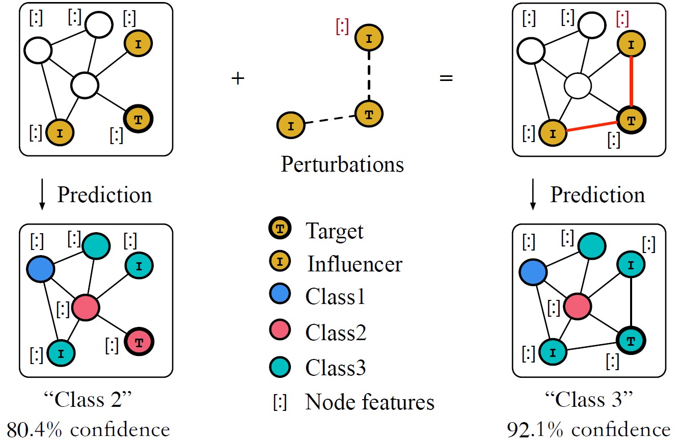
This review gives an introduction to Adversarial Machine Learning on graph-structured data, including several recent papers and research ideas in this field. This review is based on our paper “A Survey of Adversarial Learning on Graph”.