You can read the notes from the previous lecture of Chandra Chekuri's course on Count and Count-Min Sketches here.
1. Priority Sampling and Sum Queries
Suppose we have a stream a_(1),a_(2),dots,a_(n)a_{1}, a_{2}, \ldots, a_{n} (yes, we are changing notation here from mm to nn for the length of the stream) of objects and each a_(i)a_{i} has a non-negative weight w_(i)w_{i}. We want to store a representative sample S sub[n]S \subset[n] of the items so that we can answer subset sum queries. That is, given a query I sube[n]I \subseteq[n] we would like to answer sum_(i in I)w_(i)\sum_{i \in I} w_{i}. One way to do this as follows. Suppose we pick SS as follows: sample each i in[n]i \in[n] independently with probability p_(i)p_{i} and if ii is chosen we set a scaled weight hat(w)_(i)=w_(i)//p_(i)\hat{w}_{i}=w_{i} / p_{i}. Now, given a query II we output the estimate for its weight as sum_(i in I nn S) hat(w)_(i)\sum_{i \in I \cap S} \hat{w}_{i}. Note that expectation of the estimate is equal to w(I)w(I). The disadvantage of this scheme is mainly related to the fact that we cannot control the size of sample. This means that we cannot fully utilize the memory available. Related to the first, is that if we do not know the length of stream apriori, we cannot figure out the sampling rate even if we are willing to be flexible in the size of the memory. An elegant scheme of Duffield, Lund and Thorup, called priority sampling overcomes these limitations. They considered the setting where we are given a parameter kk for the size of the sample SS and the goal is maintain a kk-sample SS along with some weights hat(w)_(i)\hat{w}_{i} for i in Si \in S such that we can answer subset sum queries.
Their scheme is the following, described as if a_(1),a_(2),dots,a_(n)a_{1}, a_{2}, \ldots, a_{n} are available offline.
For each i in[n]i \in[n] set priority q_(i)=w_(i)//u_(i)q_{i}=w_{i} / u_{i} where u_(i)u_{i} is chosen uniformly (and independently from other items) at random from [0,1][0,1].
SS is the set of items with the kk highest priorities.
tau\tau is the (k+1)(k+1)'st highest priority. If k >= nk \geq n we set tau=0\tau=0.
If i in Si \in S, set hat(w)_(i)=max{w_(i),tau}\hat{w}_{i}=\max \left\{w_{i}, \tau\right\}, else set hat(w)_(i)=0\hat{w}_{i}=0.
We observe that the above sampling can be implemented in the streaming setting by simply keeping the current sample SS and current threshold tau\tau. We leave it as an exercise to show that this informatino can be updated when a new item arrives.
We show some nice and non-obvious properties of priority sampling. We will assume for simplicity that 1 < k < n1<k<n. The first one is the basic one that we would want.
Proof: Fix ii. Let A(tau^('))A\left(\tau^{\prime}\right) be the event that the kk'th highest priority among items j!=ij \neq i is tau^(')\tau^{\prime}. Note that i in Si \in S if q_(i)=w_(i)//u_(i) >= tau^(')q_{i}=w_{i} / u_{i} \geq \tau^{\prime} and if i in Si \in S then hat(w)_(i)=max{w_(i),tau^(')}\hat{w}_{i}=\max \left\{w_{i}, \tau^{\prime}\right\}, otherwise hat(w)_(i)=0\hat{w}_{i}=0. To evaluate Pr[i in S∣A(tau^('))]\operatorname{Pr}\left[i \in S \mid A\left(\tau^{\prime}\right)\right] we consider two cases.
Case 1: w_(i) >= tau^(')w_{i} \geq \tau^{\prime}. Here we have Pr[i in S∣A(tau^('))]=1\operatorname{Pr}\left[i \in S \mid A\left(\tau^{\prime}\right)\right]=1 and hat(w)_(i)=w_(i)\hat{w}_{i}=w_{i}.
Case 2: w_(i) < tau^(')w_{i}<\tau^{\prime}. Then Pr[i in S∣A(tau^('))]=(w_(i))/(tau^('))\operatorname{Pr}\left[i \in S \mid A\left(\tau^{\prime}\right)\right]=\frac{w_{i}}{\tau^{\prime}} and hat(w)_(i)=tau^(')\hat{w}_{i}=\tau^{\prime}.
In both cases we see that E[ hat(w)_(i)]=w_(i)\mathbf{E}\left[\hat{w}_{i}\right]=w_{i}.
The previous claim shows that the estimator sum_(I nn S) hat(w)_(i)\sum_{I \cap S} \hat{w}_{i} has expectation equal to w(I)w(I). We can also estimate the variance of hat(w)_(i)\hat{w}_{i} via the threshold tau\tau.
Lemma 2Var[ hat(w)_(i)]=E[ hat(v)_(i)]\mathbf{Var}\left[\hat{w}_{i}\right]=\mathbf{E}\left[\hat{v}_{i}\right]wherehat(v)_(i)={[tau max{0,tau-w_(i)},"if "i in S],[0,"if "i!in S]:}\hat{v}_{i}= \begin{cases}\tau \max \left\{0, \tau-w_{i}\right\} & \text {if } i \in S \\ 0 & \text {if } i \notin S\end{cases}
Proof: Fix ii. We define A(tau^('))A\left(\tau^{\prime}\right) to be the event that tau^(')\tau^{\prime} is the kk'th highest priority among elements j!=ij \neq i. The proof is based on showing that
In fact the previous lemma is a special case of a more general lemma below.
Lemma 4E[prod_(i in I) hat(w)_(i)]=prod_(i=1)^(k)w_(i)\mathbf{E}\left[\prod_{i \in I} \hat{w}_{i}\right]=\prod_{i=1}^{k} w_{i}if|I| <= k|I| \leq kand is 0 if|I| > k|I|>k.
Proof: It is easy to see that if |I| > k|I|>k the product is 0 since at least one of them is not in the sample. We now assume |I| <= k|I| \leq k and prove the desired claim by inducion on |I||I|. In fact we need a stronger hypothesis. Let tau^('')\tau^{\prime \prime} be the (k-|I|+1)(k-|I|+1)'th highest priority among the items j!=ij \neq i. We will condition on tau^('')\tau^{\prime \prime} and prove that E[prod_(i in I) hat(w)_(i)∣A(tau^(''))]=prod_(i in I)w_(i)\mathbf{E}\left[\prod_{i \in I} \hat{w}_{i} \mid A\left(\tau^{\prime \prime}\right)\right]=\prod_{i \in I} w_{i}. For the base case we have seen the proof for |I|=1|I|=1.
Case 1: There is h in Ih \in I such that w_(h) > tau^('')w_{h}>\tau^{\prime \prime}. Then clearly h in Sh \in S and hat(w)_(h)=w_(h)\hat{w}_{h}=w_{h}. In this case
E[prod_(i in I) hat(w)_(i)∣A(tau^(''))]=w_(h)*E[prod_(i in I\\{h}) hat(w)_(i)∣A(tau^(''))],\mathbf{E}[\prod_{i \in I} \hat{w}_{i} \mid A\left(\tau^{\prime \prime}\right)]=w_{h} \cdot \mathbf{E}[\prod_{i \in I \backslash\{h\}} \hat{w}_{i} \mid A\left(\tau^{\prime \prime}\right)],
and we apply induction to I\\{h}I \backslash\{h\}. Technically the term E[prod_(i in I\\{h}) hat(w)_(i)∣A(tau^(''))]\mathbf{E}\left[\prod_{i \in I \backslash\{h\}} \hat{w}_{i} \mid A\left(\tau^{\prime \prime}\right)\right] is referring to the fact that tau^('')\tau^{\prime \prime} is the k-|I^(')|+1k-\left|I^{\prime}\right|+1'st highest priority where I^(')=I\\{h}I^{\prime}=I \backslash\{h\}.
Case 2: For all h in I,w_(h) < tau^('')h \in I, w_{h}<\tau^{\prime \prime}. Let qq be the minimum priority among items in II. If q < tau^('')q<\tau^{\prime \prime} then hat(w)_(j)=0\hat{w}_{j}=0 for some j in Ij \in I and the entire product is 0. Thus, in this case, there is no contribution to the expectation. Thus we will consider the case when q >= tau^('')q \geq \tau^{\prime \prime}. The probability for this event is prod_(i in I)(w_(i))/(tau^(''))\prod_{i \in I} \frac{w_{i}}{\tau^{\prime \prime}}. But in this case all i in Ii \in I will be in SS and moreover hat(w)_(i)=tau^('')\hat{w}_{i}=\tau^{\prime \prime} for each ii. Thus the expected value of prod_(i in I) hat(w)_(i)=prod_(i in I)w_(i)\prod_{i \in I} \hat{w}_{i}=\prod_{i \in I} w_{i} as desired.
Combining Lemma 2 and 3 the variance of the estimator sum_(i in I nn S) hat(w)_(i)\sum_{i \in I \cap S} \hat{w}_{i} is
Var[sum_(i in I nn S) hat(w)_(i)=sum_(i in I nn S)Var[ hat(w)_(i)]=sum_(i in I nn S)E[ hat(v)_(i)].\mathbf{Var}[\sum_{i \in I \cap S} \hat{w}_{i}=\sum_{i \in I \cap S} \mathbf{Var}\left[\hat{w}_{i}\right]=\sum_{i \in I \cap S} \mathbf{E}\left[\hat{v}_{i}\right] .
The advantage of this is that the variance of the estimator can be computed by examining tau\tau and the weights of the elements in the S nn IS \cap I.
2. ℓ_(0)\ell_{0} Sampling
We have seen ℓ_(2)\ell_{2} sampling in the streaming setting. The ideas generalize to ℓ_(p)\ell_{p} sampling to ℓ_(p)\ell_{p} sampling for p in(0,2)p \in(0,2) – see [] for instance. However, ℓ_(0)\ell_{0} sampling requires slightly different ideas. ℓ_(0)\ell_{0} sampling means that we are sampling near-uniformly from the distinct elements in the stream. Surprisingly we can do this even in the turnstile setting.
Recall that one of the applications we saw for the Count-Sketch is ℓ_(2)\ell_{2}-sparse recovery. In particular we can obtain a (1+epsilon)(1+\epsilon)-approximation for err_(2)^(k)(x){ }_{2}^{k}(\mathbf{x}) with high-probability using O(k log n//epsilon)O(k \log n / \epsilon) words. Suppose x\mathbf{x} is kk-sparse then err _(2)^(k)(x)=0{ }_{2}^{k}(\mathbf{x})=0! It means that we can detect if x\mathbf{x} is kk-sparse, and in fact identify the non-zero coordinates of x\mathbf{x}, with high-probability. In fact one can prove the following stronger version.
Lemma 5For 1 <= k <= n1 \leq k \leq n there and k^(')=O(k)k^{\prime}=O(k) there is a sketch L:R^(n)rarrR^(k^('))L: \mathbb{R}^{n} \rightarrow \mathbb{R}^{k^{\prime}} (generated from O(k log n)O(k \log n) random bits) and a recovery procedure that on input L(x)L(\mathbf{x}) has the following feature: (i) if x\mathbf{x} is kk-sparse then it outputs x^(')=x\mathbf{x}^{\prime}=\mathbf{x} with probability 1 and (ii) if x\mathbf{x} is not kk-sparse the algorithm detects this with high-probability.
We will use the above for ℓ_(0)\ell_{0} sampling as follows. We will first describe a high-level algorithm that is not streaming friendly and will indicate later how it can be made stream implementable.
For h=1,dots,|__ log n __|h=1, \ldots,\lfloor\log n\rfloor let I_(h)I_{h} be a random subsets of [n][n] where I_(j)I_{j} has cardinality 2^(j)2^{j}. Let I_(0)=[n]I_{0}=[n].
Let k=|~4log(1//delta)~|k=\lceil 4 \log (1 / \delta)\rceil. For h=0,dots,|__ log n __|h=0, \ldots,\lfloor\log n\rfloor, run kk-sparse-recovery on x\mathbf{x} restricted to coordinates of I_(h)I_{h}.
If any of the sparse-recoveries succeeds then output a random coordinate from the first sparserecovery that succeeds.
Algorithm fails if none of the sparse-recoveries output a valid vector.
Let JJ be the index set of non-zero coordinates of x\mathbf{x}. We now show that the algorithm with probability (1-delta)(1-\delta) succeeds in outputting a uniform sample from JJ. Suppose |J| <= k|J| \leq k. Then x\mathbf{x} is recovered exactly for h=0h=0 and the algorithm outputs a uniform sample from JJ. Suppose |J| > k|J|>k. We observe that E[|I_(h)nn J|]=2^(h)|J|//n\mathbf{E}\left[\left|I_{h} \cap J\right|\right]=2^{h}|J| / n and hence there is a h^(**)h^{*} such that E[|I_(h^(**))nn J|]=2^(h^(**))|J|//n\mathbf{E}\left[\left|I_{h^{*}} \cap J\right|\right]=2^{h^{*}}|J| / n is between k//3k / 3 and 2k//32 k / 3. By Chernoff-bounds one can show that with probability at least (1-delta)(1-\delta), 1 <= |I_(h^(**))nn J| <= k1 \leq\left|I_{h^{*}} \cap J\right| \leq k. For this h^(**)h^{*} the sparse recovery will succeed and output a random coordinate of JJ. The formal claims are the following:
With probability at least (1-delta)(1-\delta) the algorithm outputs a coordinate i in[n]i \in[n].
If the algorithm outputs a coordinate ii then the probability that it is not a uniform random sample is because the sparse recovery algorithm failed for some hh; we can make this probability be less than 1//n^(c)1 / n^{c} for any desired constant cc.
Thus, in fact we get zero-error ℓ_(0)\ell_{0} sample.
The algorithm, as described, requires one to sample and store I_(h)I_{h} for h=0,dots,|__ log n __|h=0, \ldots,\lfloor\log n\rfloor. In order to avoid this we can use Nisan's pseudo-random generator for small-space computation. We skip the details of this; see[1]. The overall space requirements for the above procedure can be shown to be O(log^(2)n log(1//delta):}O\left(\log ^{2} n \log (1 / \delta)\right. with an error probability bounded by delta+O(1//n^(c))\delta+O\left(1 / n^{c}\right). This is near-optimal for constant delta\delta as shown in[1:1].
Bibliographic Notes: The material on priority sampling is directly from[2] which describes applications, relationship to prior sampling techniques and also has an experimental evaluation. Priority sampling has shown to be "optimal" in a strong sense; see[3].
The ℓ_(0)\ell_{0} sampling algorithm we described is from the paper by Jowhari, Saglam and Tardos[1:2]. See a simpler algorithm in the chapter on signals by McGregor-Muthu draft book.
You can read the notes from the next lecture of Chandra Chekuri's course on Quantiles and Selection in Multiple Passes here.
Hossein Jowhari, Mert Saglam, and Gábor Tardos. Tight bounds for lp samplers, finding duplicates in streams, and related problems. CoRR, abs/1012.4889, 2010. ↩︎↩︎↩︎
Nick Duffield, Carsten Lund, and Mikkel Thorup. Priority sampling for estimation of arbitrary subset sums. Journal of the ACM (JACM), 54(6):32, 2007. ↩︎
Mario Szegedy. The dlt priority sampling is essentially optimal. In Proceedings of the thirtyeighth annual ACM symposium on Theory of computing, pages 150-158. ACM, 2006. ↩︎
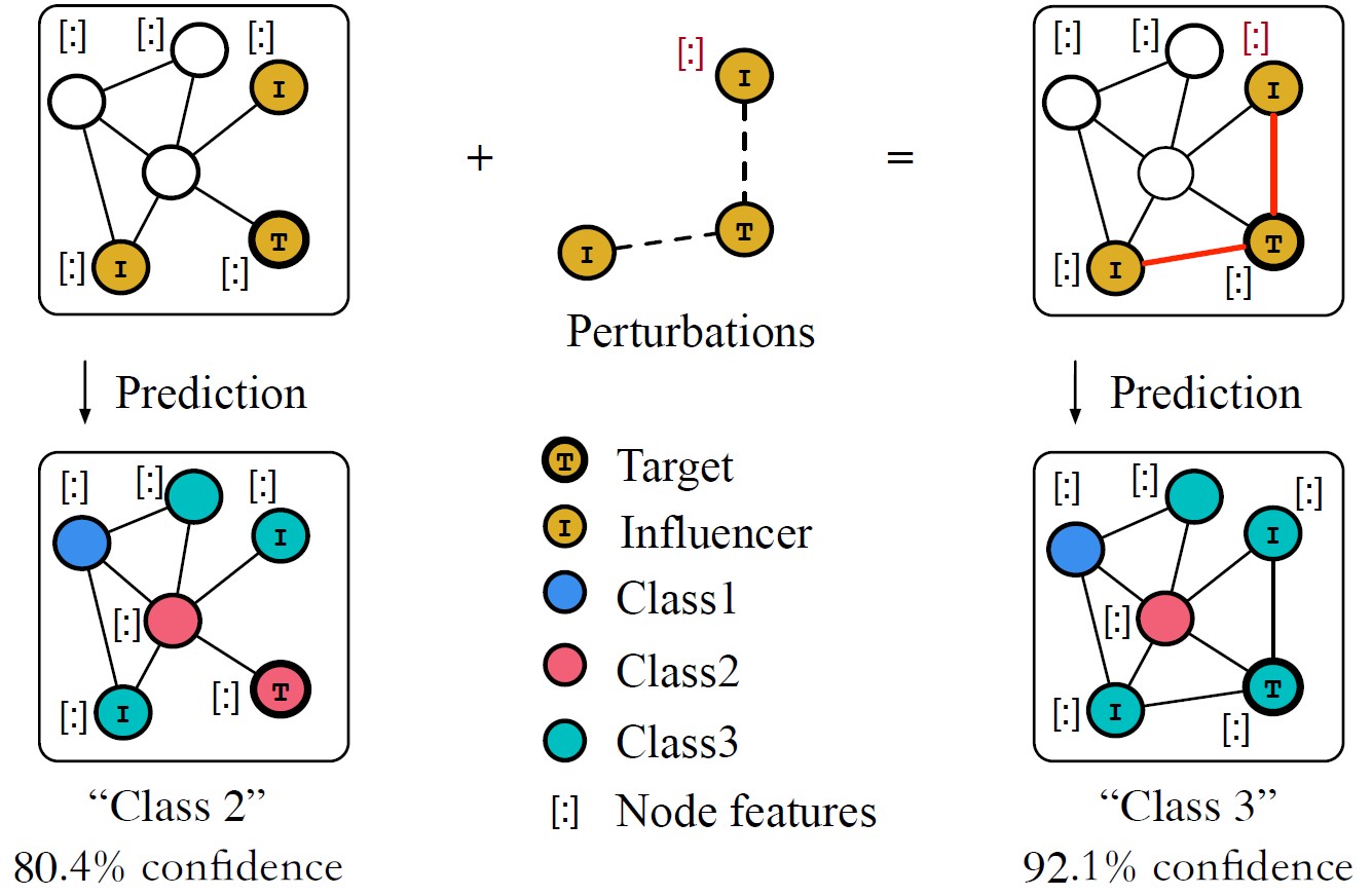
This review gives an introduction to Adversarial Machine Learning on graph-structured data, including several recent papers and research ideas in this field. This review is based on our paper “A Survey of Adversarial Learning on Graph”.