Text Generation Models - Introduction and a Demo using the GPT-J model
Natural Language Modelling is a computational technique in the realm of software engineering and Artificial Intelligence that helps us manage, represent and analyze human languages. Text generation is a computational linguistic tool that enables us to generate new grammatically and semantically correct synthetic text. The text uses input in the form of natural language text, numerical data or even a line of code (example: often phrases or sentences that act as the starting phrase of a piece of text or even data that can be built into natural readable text). A text generation model takes input data, learns the context from the input, and generates new text relating to the domain of input data. The generated text should satisfy the basic language structure and convey the desired message, often adhering to other parameters provided while training the model or during inference, like the length of the generated text, vocabulary size etc. Text generation can be a complicated process as it is difficult to evaluate the grammatical, semantic, and logical accuracy of the generated text. Although there are a few metrics now, to evaluate the results of a text generation model, there is no absolute way to determine the best solution. We will cover some of these metrics later in this article.
1. What is Text Generation?
Text generation is an application of a causal language model. A language model is a probabilistic statistical model that determines the probability of a given sequence of words occurring in a sentence based on the other words in the text and regular patterns in the human language. There are 2 main kinds of language models: Causal Language Model and Masked Language Model. A causal language model (CLM) is a unidirectional model that predicts a masked token (or word) in a given sentence, considering the words that occur to its left. This is a unidirectional model (and hence ideally, the words in only one direction will be considered) that checks the prediction made by the model against the actual label, calculates cross-entropy loss and backpropagates it to train the model parameters.
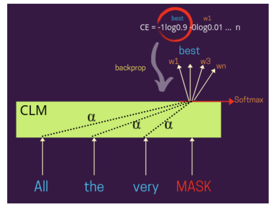
In the above image, we see that the we can weigh the representation of every other input word using the distribution of
Masked Language models (MLMs), like CLMs, are also used to predict masked words based on other words in that sentence. However, the difefrence is that these are bidirectional models which means that they consider surrounding words both on the left and on the right of the masked token. Below is an image that represents the training mechanism for MLMs which is very similar to that of the CLMs.
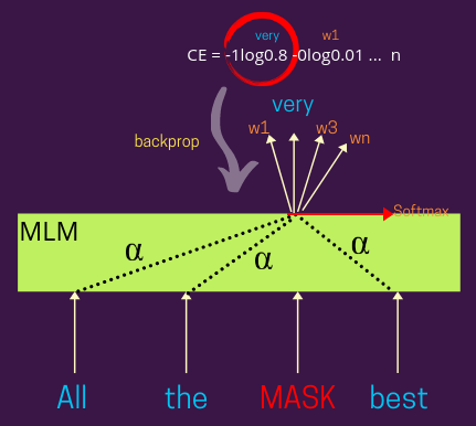
MLM representations can also be learnt using both attention-based architectures like BERT or even simpler conventional algorithms.
Text generation is an example of a causal language model that uses the input text to learn the representations and then generate the next token on the basis of the learnt representations. This way it aims to generate text that replicates natural human language.
Most advanved deep-learning based text-generation models can be classified as below:
- Vector-Sequence Model – These models use a fixed-size vector input whereas output can vary. Such a model is widely used for caption generation of images [1].
- Sequence-Vector Model - These models use inputs of variable size, and the output is a fixed-size vector. A prominent example of such a model is text classification [2].
- Sequence-to-Sequence Model - These models use variable-sized inputs and outputs. While it is the most widely used variant of text generation models, one common application of such models is language translation [3].
Text generation can be performed at different granularity of text, i.e., at a character, word, and sentence level. At a sentence level, the text-generation model aims to analyze the entire text as a finegrained entity and learns the relationship between the sentence and its context. On the other hand, word-based text generation seeks to explore the structure of a sequence and predict the probability of the next word in a given text. Similarly, the model identifies the character rather than the entire document at character level text generation.
1.1. Use Cases of Text Generation
Text generation has a lot of direct use-cases like code generation, and stories-generation. For code generation, the model is trained on code from scratch. The models generate code that can help programmers with their repetitive and standardized programming tasks. For story generation, we can provide input phrases like "Once upon a time" and models like GPT-2[4] can be trained to generate numerous stories with that beginning. Some of the more common applications can be prediction of next word while using the chatting functionality on your phones.
2. Text Generation using Markov Chains
Markov Chains [5] are mathematical models that represent and manage stochastic processes and predict the condition of the next state based on condition of the previous state. It is called as a stochastic process because it changes or evolves over time. Let us look at the below diagram.
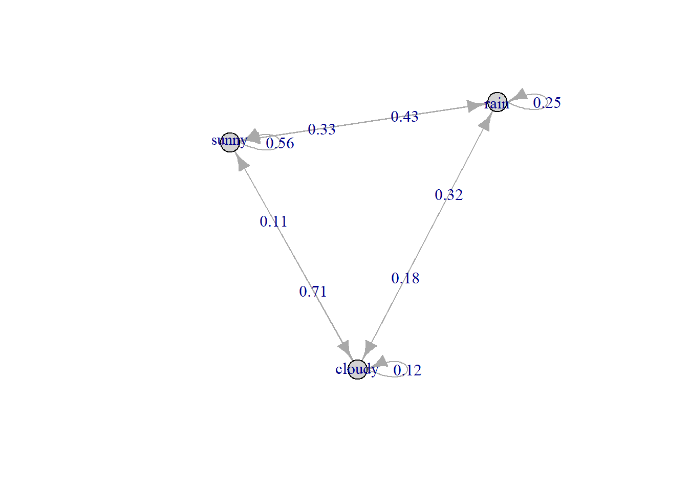
In the image above, we see that there are three possible states: sunny, rainy, and cloudy. Say if the current state is sunny, there is a 56% probability of it being sunny the next day. The probability of it being cloudy is 11% and that of raining is 33%.
These probabilities are called transition probabilities. The default method to calculate the transition probability is by using Maximum Likelihood Method (MLE) by using the following equation:
Here,
We can also add a laplace smoothing term to avoid zero-probabilities:
Here
Using Markov Chains for text generation has a few benefits like low computation time and space complexity as well as the simple interpretation and implementation of these models. However, there are also a few disadvantages:
- The quality of the generated text is a direct function of the input corpus. If the training text is not logically, semantically and grammatically accurate, the generate text will also not be very sound.
- Moreover, since the next state only depends on the current state and independent from the past (i.e. Lack of Memories), it is difficult to set context or assign necessary weights to certain parts of the input text. This might lead to low quality predictions.
- To teach context to a Markov Chain, we need to create a higher order model by training multiple n-gram Markov Chains, which may increase the complexity too.
3. Text Generation using Deep Learning Models
Deep learning models can also be used to generate text. They can generate more grammatically and semantically accurate text, but come with higher time and space complexity. One of the simpler deep learning models are Recurrent Neural Networks (RNNs). RNN is a class of neural networks that uses the output of previous states as input in future states. It is the first algorithm that preserves the outputs of past states. However, it forgets the previous outputs over a period of time due to a vanishing gradient. This might lead to failure in capturing broader context and information that is distant from the masked token (i.e. the token to be predicted). One special class of RNN is Long Short Term Memory (LSTM) [6] which we will briefly cover below.
3.1. LSTM
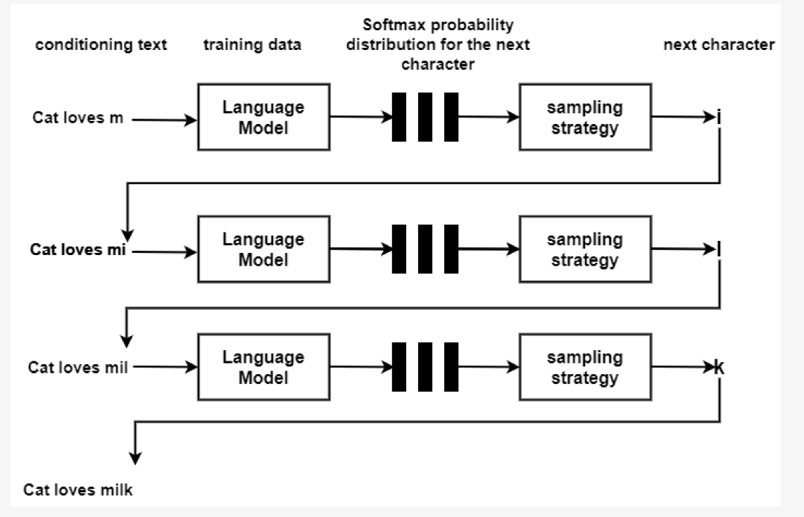
LSTM is a special kind of RNNs that overcome the issue of vanishing gradient of RNNs. LSTM retains information of previous states over a very long period and forgets the irrelevant information. The LSTM model is trained on Wikipedia text or domain knowledge from the conditioning text.
To predict the probability of the next character using the Softmax activation function at the output layer is defined as below:
Here,
We define the term
where
where
However, studies have notices that the generated text obtained from LSTM presents local coherence but it lacks logic.
Below is an example of the output of text generation using LSTM with varying temperature values:

We see that as the temperature increases, the vocabulary becomes richer and the results become more surprsing. However, we see that the results do not make logical sense and are also not accurate grammatically.
To make further improvements, we can look into Transformer-based models like GPT or BERT.
3.2. BERT
BERT or BiDirectional Encoder Representations from Transformers are tranformer-based models used for a wide variety of deep learning applications. To understand BERT better, let us try to understand the Transformer architecture first. Below is a graphical representation of the transformer architecture:
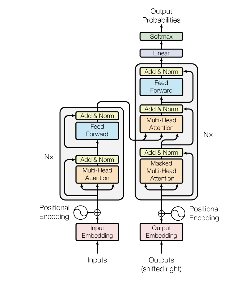
A typical transformer model has an encoder-decoder structure. Without getting too much into the details of the encoder and decoder itself , let us understand another significant part of the transformer models: Attention [7].
3.2.1. Attention Mechanism
An attention function can be described as a mapping between a query and a set of key-value pairs to an output. Here, the query, keys, values, and output are all vectors. The output of attention is a weighted sum of the values, where the weight assigned to each value can be computed by a compatibility function of the query with the corresponding key. In simpler terms, attention is memory per unit of time. The weights assigned to the inputs above define how important certain parts of the input are. Thus, using attention we can focus on a certain component of the input problem and take greater notice of it. This is particularly helpful in text and NLP applications where you want to stress on some parts of the text to give them more importance in setting context. For example, in text translation tasks like translating "I hope you are doing well" to Spanish, we map the input sequence "I hope" to a single Spanish word "Espero". Thus, higher 'weights' or relevance assigned to certain input sequence words help us get an accurate relation to the appropriate words in the output sequence. This enhances the accuracy of output prediction as the attention model is more capable of producing relevant output.
3.2.2. BERT model
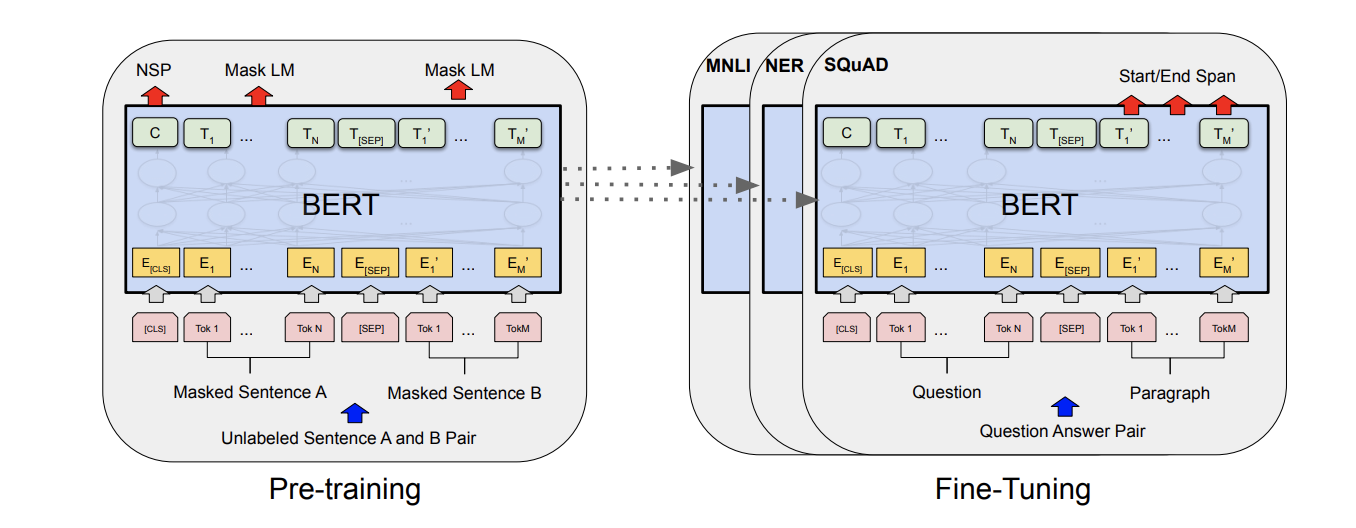
The above image shows that there are two main parts to the BERT framework:
- Pre-training which includes training the model on unlabeled data over different pre-training tasks like Masked LM and Next Sentence Prediction. The authors pretrained BERT on the BooksCorpus and Wikipedia
- Finetuning the model involves a transfer learning [8] process wherein it is initialized with the pre-trained parameters. Then, the model is fine-tuned for each downstream task separately.
To understand how BERT can be used for language generation, we first need to note that it uses the Masked Language Model method. [CLS], [SEP] and [MASK] are the three important tokens in the BERT mechanism. [CLS] defines a class that holds the embedding representation of full input context rather than any specific word. [SEP] token is a separator tag that helps the model to separate out two sentences in the input and also as end token for any sentence. Lastly, [MASK] token is the placeholder for the masked token that the model tries to predict based on context words.
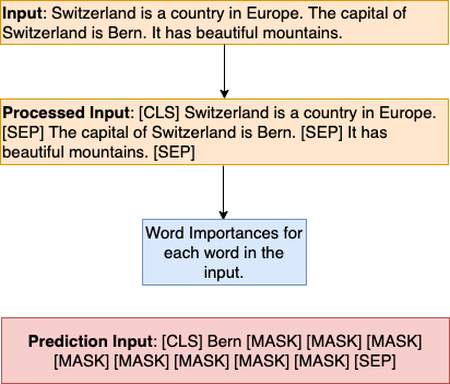
Let us look at the image above. The BERT model learns the importance of all the words from the input. We can then prompt the model to generate text with asimilar format. However, since BERT is trained using MLM (masked language model) which is bidirectional, it uses the Random Hop Generation Strategy to generate text.
In this strategy, we iterate over the prediction input
The other strategy is an autoregressive Left to Right Generation Strategy where the model always predicts the [MASK] that is at extreme right based on the context words that have been filled on the left. That is ideally how text generation works. However, since BERT has been trained using MLM, and not the typical autoregressive style, it is not the best model for text generation. BERT works better in use cases where a percentage of input tokens are masked at random and only those tokens are predicted based on remaining words. Since the given words lie both to their left and right ,it lends a rich bidirectional context to the masked token.
Some other transformer based-models that work better for text generation are GPT-2 [9] or even GRU-based language models [10]. Let us talk about the GPT model in detail below.
3.3. GPT-2
Generative Pretrained Transformer 2, known by GPT-2, is a large unsupervised transformer-based language model which was developed as a successor to GPT [11]. The authors of GPT-2 trained it with the objective of predicting the next word, given some input text. In terms of its architecture, it is a stack of decoders, and thus aligns with the basic definition of a causal language model (text generation particularly).
Like most other transformer-based models, GPT-2 also has two steps in the training process:
- Pretraining: Here the language model is trained on a huge corpus of text data from the internet.
- Finetuning: Here we tune and adapt the model to the specific task.
In the pretraining stage, we use a standard language modeling objective to maximize the following likelihood:
Given,
Here
After the pretraining process as per the equation above, the next step is supervised fine-tuning. Assuming we have a dataset
The final maximization objective is then as follows:
At the end of the two steps, for most language modelling tasks the aim is to improve the generalization of the supervised model. Effectively, the final objective is as follows:
where
For text generation, we know that GPT-2 has been trained conventionally like a decoder and can generate text based on the input text. The longer an initial input piece of text is, the more subject context is provided to the model. In most cases, longer inputs produce a more coherent text output.
Owing to the auto-regressive nature of the text generation process, GPT-2 makes it possible to generate long chunks of contextually coherent and often semantically and grammatically accurate (as comapred to natural human language) paragraphs of text. Moreover, since self-attention [7] is an important part of GPT-2 models. This helps the model to relate different positions of a specific sequence of input tokens in order to compute a contextual representation of the sequence. This makes GPT-2 one of the State of The Art models with promising results in predicting the next word by the given context.
4. Prototype: Domain-Specific Text Generation for Machine Translation
Some of the recent language models have been developed to work with text of particular domain. It is important to train a model on the relevant context to generate correct and logical results, pertaining to a particular industry or subject. For specialized projects, these models have been trained with mixed fine-tuning that significantly improve translation of in-domain texts [12].
These highly trained specialized frameworks employ large models like GPT-J. The GPT-J model was released in the Ben Wang and Aran Komatsuzaki (Source: https://github.com/kingoflolz/mesh-transformer-jax). It finds application a lot of tasks like translation, question answering, text generation etc. The authors address the GPT-J model also as GPT-J-6B as it is a large model trained using 6 billion parameters. It is an autoregressive text generation model trained on The Pile [13] training set.
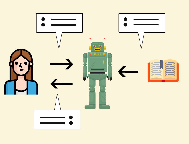
Let us go through a quick demo of using GPT-J to generate text given the first text as prompt. Below is a snapshot to show the Python execution of the process of downloading the GPT-J model and loading it correctly onto the GPU environment for text generation.
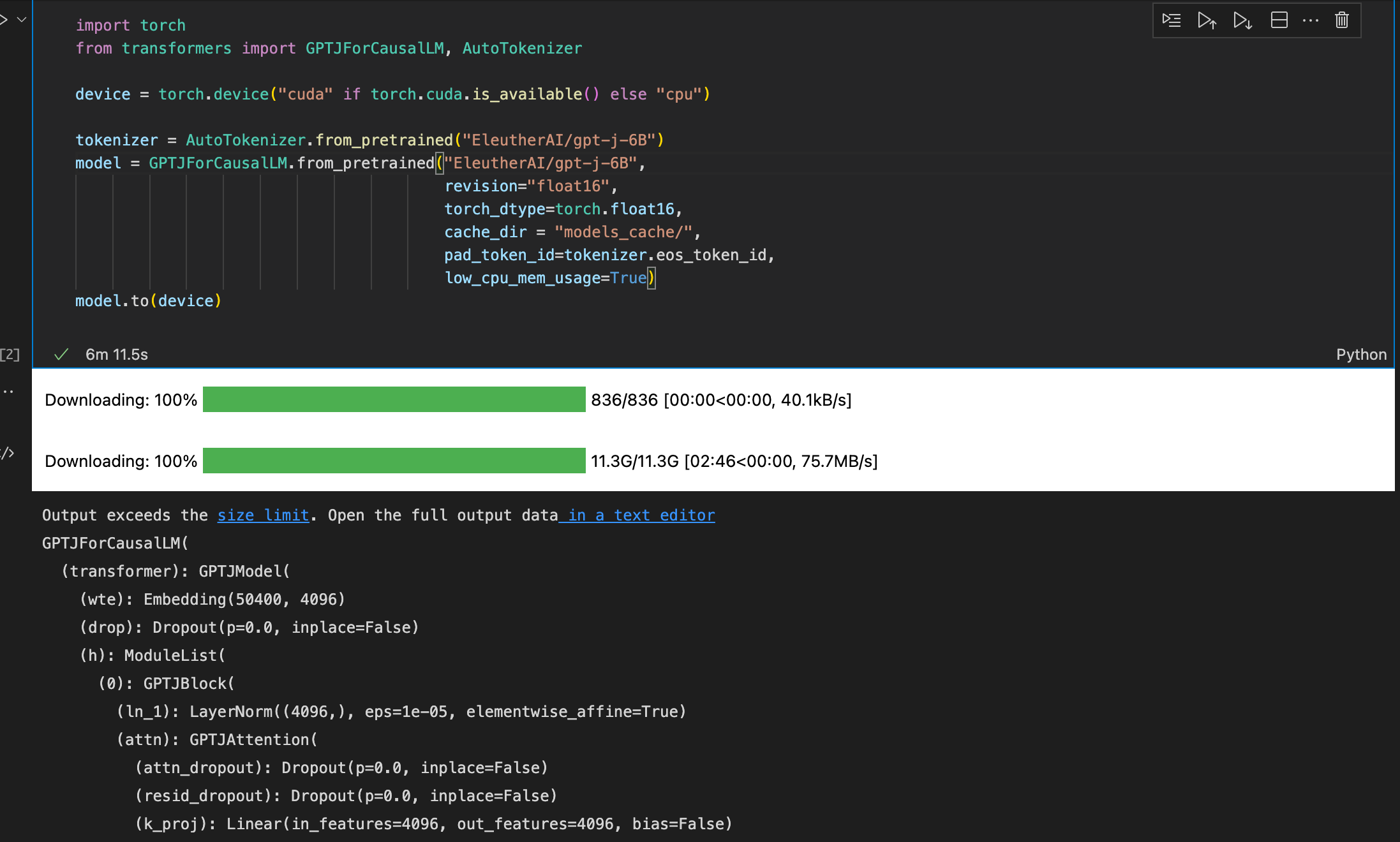
We see that the model size is large (~12 GBs) and owing to the time and space complexity, it is recommended to use this model on a GPU.
The next step is to pass a text file as an input to the model. In this text (.txt) file, we provide 3 different sentences on unrelated topics as input prompts for the model to generate more text on.

As we see above, the three sentences are about a Google product launch, environmental development and image generation using AI respectively.
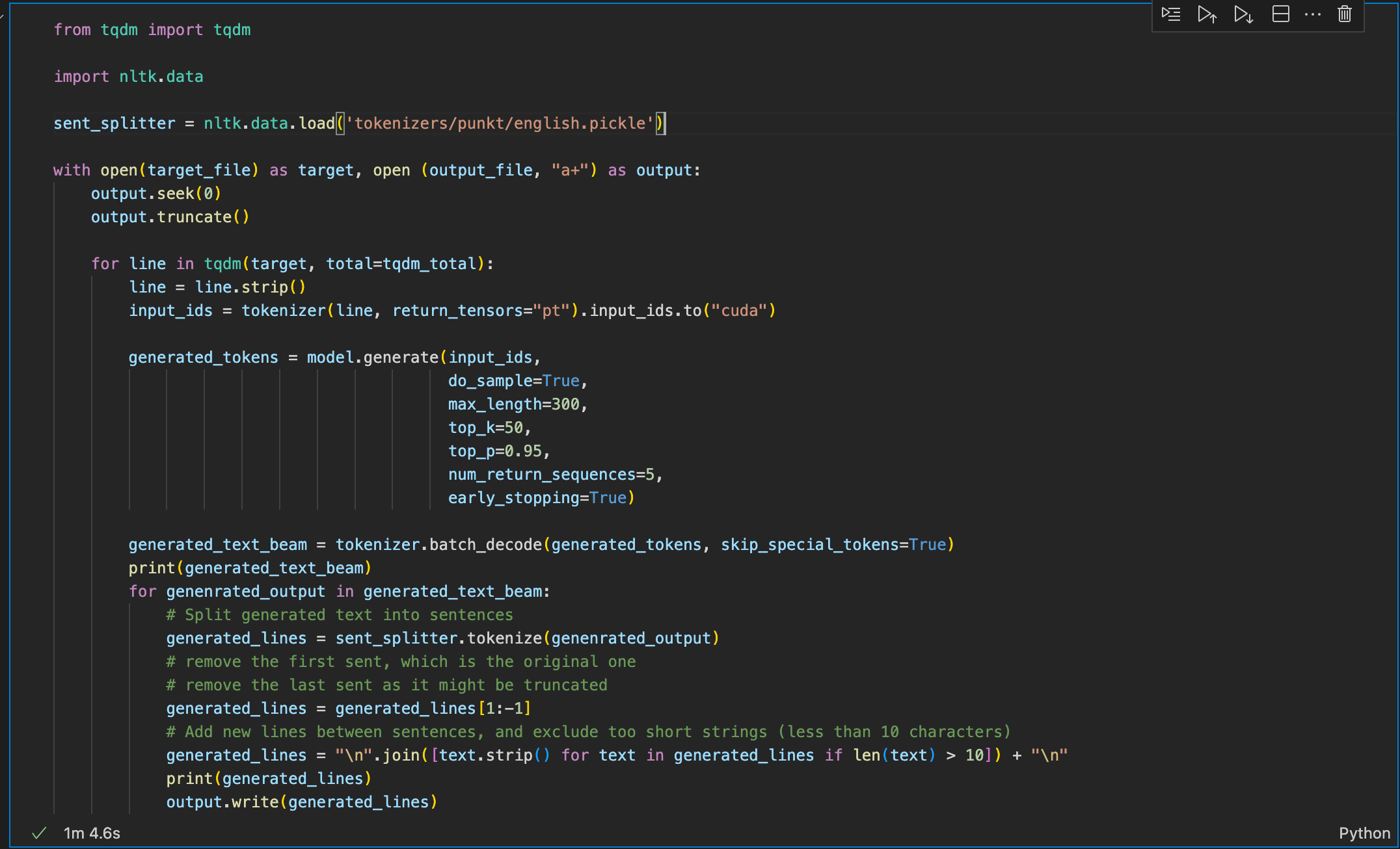
The final step was to pass these inputs onto the loaded model for text generation. We also pass parameters to define how we want the output to be:
Here,
max_length: defines the maximum length the generated text can have. This includes the length of the input text. We also have another possible parameter called max_new_tokens which defines the number of new tokens that the model can generate. In general,
do_sample: specifies whether or not to use sampling; The model would use greedy decoding if set to False.
top_k: The number of highest probability vocabulary tokens to keep for top-k-filtering. This means that the
There is another method of text sampling which can also be passed as a parameter here: temperature. This parameter enables us to perform temperature sampling, where high temperature means low energy states are more likely encountered. In probabilistic models, logits equate to energy and we can implement temperature sampling by dividing logits by the temperature before feeding them into softmax and obtaining our sampling probabilities. A higher temperature would a more fiverse and larger vocabularythus making the results more surprising. In most cases, either of the top-k and temperature are used to achieve the desired results.
top_p: If set to float < 1, only the most probable tokens with probabilities that add up to top_p or higher are kept for generation. Top-P Sampling is another sampling method that aggregates the smallest set of words which have a summed probability mass
num_return_sequences: The number of independently computed returned sequences for each element in the batch. This is the parameter that defines the number of different sequences (or text pieces) you want to generate from the same input text. The corresponding number of higher scoring sequences will be returned.
Let us look at the output of each input string:
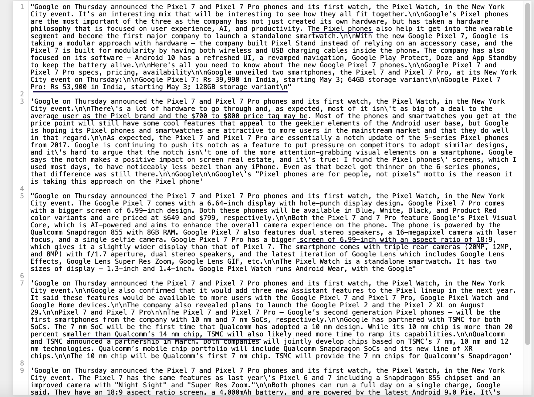
Looking at the 5 outputs for the input string:
Google on Thursday announced the Pixel 7 and Pixel 7 Pro phones and its first watch, the Pixel Watch, in the New York City event.
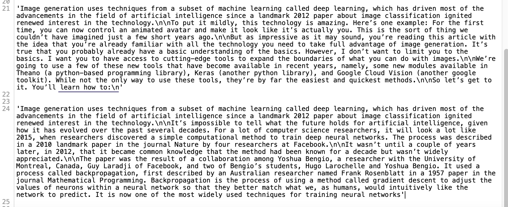
We see that though most of the outputs have coherence and a general semantic and grammatical accuracy, the generated text also has some facts, numbers and specifics that may or may not be accurate (could be fictional too!). Some of these facts that have been incorporated (see underlined text in the snapshot above) in the generated text needs to be checked for and corrected, if needed before using the information any further. However, it is impressive how the sentences are coherent and talk about the particular domain given in the input sentence. To show how the model works across inputs of different domains, let us also look at the outputs for the next 2 input samples:
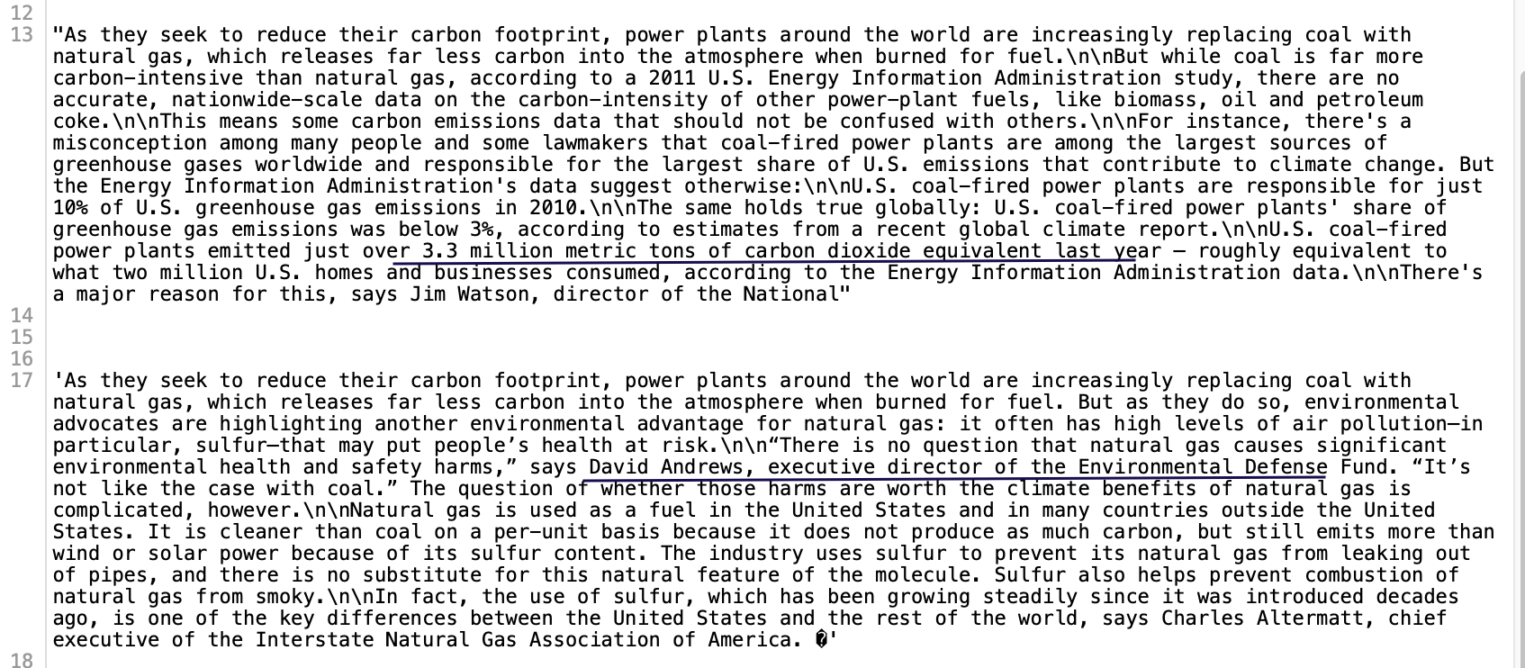
Again, we see facts that sound correct but need to be checked for factual accuracy. However, we see that the text generated is logical, coherent and relevant to the input text that was provided to the model. We see a simiar trend with the last example. We see that some times, the generated text ends abruptly (in the image below). That can be controlled for, using the max_length parameter.
5. A quick review of other advanced techniques
5.1. Knowledge-Enhanced Text Generation
Before getting into the methods, let us understand what knowledge-enhanced text generation is. Knowledge, in the simplest terms can be defined as the familiarity, awareness, or understanding around a particular subject or domain. In natural language systems, knowledge represents understanding of the input text and its surrounding context. The knowledge sources can be categorized into two types:
- Internal sources: This entails the knowledge contained in the input text which includes keyword, topic, linguistic features, and internal graph structure.
- External sources: We can obtain external knowledge from sources like knowledge base, external knowledge graph, and grounded text.
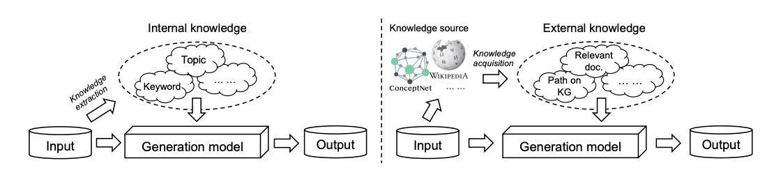
This knowledge sourced from various sources can help the learning process for neural systems and thus also improve the text generation process. This line of research is called knowledge-enhanced text generation. The image above shows the basic process of sourcing knowledge from internal and external sources and using it to generate text.
The problem can be defined as follows:
A text generation problems has been given an input sequence
A major component of the knowledge-enhanced text generation models is the attention mechanism. It captures the weight of each time step in both encoder and decoder. The general idea behind knowledge-related is to learn a knowledge-aware context vector by combining both the hidden context vector and the knowledge context vector. The knowledge context vector calculates calculates attentions over knowledge representations (e.g., topic vectors, keyword vectors, node vectors in knowledge graph), and hence factors in keyword attention, topic attention, knowledge base attention, knowledge graph attention, and grounded text attention.
The next important component is Copy and Pointing Mechanisms. CopyNet and Pointer-generator (PG) are used to select sub-sequences in the input sequence and put them at proper places in the output sequence. This leads to a combined probability of generating a target token factoring in the probabilities of two modes: generate-mode and copy-mode. The objective of using these mechanisms is to build an extended vocabulary for the model by combining the vocabulary of source sequence and the global vocabulary. It is particularly useful for Language Generation models to generate words that are not included in the global vocabulary (
Memory networks and graph networks are also vital in this process. Memory networks are recurrent attention models over
a possibly large external memory. It enables us to encode long dialog history and memorize external information. Literature shows that memory augmented encoder-decoder frameworks have been incorporated in language models and have showed promising results. For example, they can help in tasks where we need to memorize dialogue history, like in task-oriented dialogue systems [16]. Such frameworks enable a decoder to retrieve information from a memory during generation.
Graph networks can be used to integrate knowledge in graph structure such as knowledge graph and dependency graph. A graph attention network,combined with sequence attention and jointly optimized can enhance the results obtained from a language generation model [17]. Using knowledge graphs, multiple property fields like data attributes or facts and their corresponding values can be integrated into the generated text. This finds application in generating text for factual reports etc.
5.2. Layer-Wise Latent Variable Inference for Text Generation
In 2022, Jinyi Hu et al. proposed a novel method to incorporate latent variables in simple language generation tasks and introduced a variational Transformer framework called "DELLA" [18]. This model tackles the problem of KL vanishing. Let us first try to understand what KL vanishing is. VAEs or variational autoencoders are models trained with one core objective: to represent the original data best with a minor loss of information. The objective function consists of two terms:
Here, the first term is the reconstruction loss while the second term is the loss of Kullback–Leibler divergence term (KL loss). While the first term indicates how well a VAE can reconstruct the input sequence from the latent space, the latter measures how similar two data distributions are with each other. The objective is to reduce the KL-loss so:
where we want to ensure that
DELLA, however learns a series of layer-wise latent variables with each inferred from those of lower layers and tightly coupled with the hidden states. This way, it incorporates the posterior latent variables with the whole computation path deeply and hence incorporates more information.
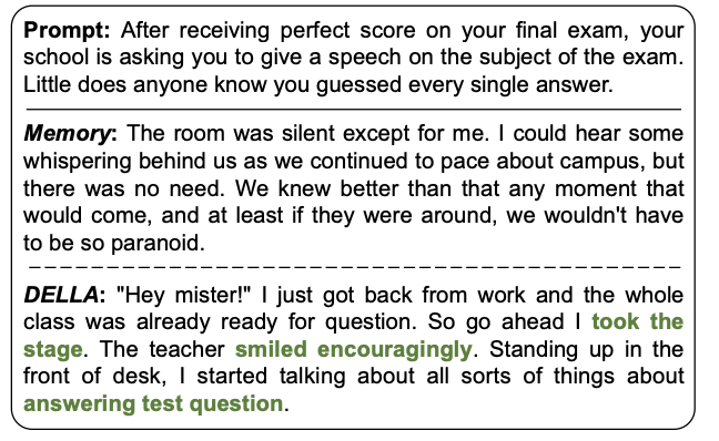
If we look at the example above, we see that the generated text from Memory, is not related to the prompt and is meaningless. However, the DELLA framework LLA generates coherent and vivid text w.r.t the prompt.
6. Metrics for evaluating Text Generation Models
As mentioned earlier, there is no determinsitic metric that can measure the performance of natural language models. Generated text cannot be measured for absolute accuracy. However, it can be evaluated for its semantic richness, and logical and grammatical correctness. Some of these metrics that vare commonly used in this context are described below.
6.1. Recall Oriented Understudy for Gisting Evaluation (ROUGE)
This metric is more relevant in cases when there is a base truth against which the generated text can be compares. Text summarization is the one application that can be evaluated using the Rouge materic. Please note that this measure would not be very helpful metric in unsupervised applications where there is not base golden truth to compare the system-generated text against.
The Rouge score measures the similarity between the reference summary (golden summary) and the system-generated summary. Let us cover a few metrics that help make up the metrics that we will cover further below:
- Recall:- It indicates how much of the golden summary the generated summary captures. It is calculated as:
- Precision: It indicates the system summary which is relevant or needed and is calculated as:
Using the above definition of recall, Rouge score can be extended as Rouge-1 and Rouge-2 score for evaluating unigrams and bigrams respectively. Generally, Rouge-n can be used for matching n-grams in the 2 summaries.
6.2. Bilingual Evaluation Under-study (BLEU)
BLEU is another metric that evaluates a generated text piece against reference text. It is importance to note that the Bleu Score is calculated by considering the text of the entire predicted corpus as a whole. We cannot calculate the Bleu score separately on each sentence in the corpus, and then average those scores in some way.
It measures how much the words (and/or n-grams) in the machine generated summaries appear in the human reference summaries or the golden summary. The difference between Rouge and BLEU is that while Rouge measures recall (i.e. how much the words (and/or n-grams) in the human reference summaries appeared in the machine generated summaries), BLEU measures the precision.
The BLEU score incorporates a component called brevity penalty which can be defined as below:
where
6.3. Word perplexity (PPL)
Word perplexity pr perplexity is a commonly used metric for language models. It can be defined as:
where
To interpret the PPL score, let us look at this sentence as an example input prompt: The latest report on global economy says____
A better language model would generate a meaningful sentence for the above prompt by placing a word based on conditional probability values which were assigned using the training corpus. Hence, we can say that how well a language model can predict the next word and therefore make a meaningful sentence is asserted by the perplexity value assigned to the language model based on a test set.
Thus, better language models will have lower perplexity values or higher probability values for a test set.
7. References
- M. Toshevska, F. Stojanovska, E. Zdravevski, P. Lameski, and S. Gievska, ‘‘Explorations into deep learning text architectures for dense image captioning,’’ (2020).
- O. Abdelwahab and A. Elmaghraby, ‘‘Deep learning based vs. Markov chain based text generation for cross domain adaptation for sentiment classification,’’ (2018)
- O. Dušek, J. Novikova, and V. Rieser, ‘‘Evaluating the state-of-the-art of end-to-end natural language generation: The E2E NLG challenge,’’ (2020).
- Radford, Alec et al. “Language Models are Unsupervised Multitask Learners.” (2019).
- Yang, Xinye and Yang, Xinye, ‘‘Markov Chain and Its Applications” (2019)
- S. Hochreiter and J. Schmidhuber, ‘‘Long short-term memory,’’ (1997).
- Vaswani A. et al. ‘‘Attention Is All You Need’’ (2017)
- F. Zhuang et al. ‘‘A Comprehensive Survey on Transfer Learning’’ (2020)
- Radford A. et al. ‘‘Language Models are Unsupervised Multitask Learners’’ (2018)
- Li X. et al. ‘‘Multi-Modal Gated Recurrent Units for Image Description’’ (2019)
- Radford A. et al. ‘‘Improving Language Understanding by Generative Pre-Training’’ (2018)
- Yasmin Moslem, Rejwanul Haque, John Kelleher, Andy Way ‘‘Domain-Specific Text Generation for Machine Translation’’ (2022)
- The Pile training set: https://pile.eleuther.ai/
- Fan A. et al. ‘‘Hierarchical Neural Story Generation’’ (2018)
- Yu W. et al. ‘‘A Survey of Knowledge-Enhanced Text Generation’’ (2022)
- Revanth Gangi Reddy, Danish Contractor, Dinesh Raghu, and Sachindra Joshi, ‘‘Multi-Level Memory for Task Oriented Dialogs.’’ (2019)
- Rik Koncel-Kedziorski, Dhanush Bekal, Yi Luan, Mirella Lapata, Hannaneh Hajishirzi ‘‘Text Generation from Knowledge Graphs with Graph Transformers.’’ (2019)
- Hu J. et al. ‘‘Fuse It More Deeply! A Variational Transformer with Layer-Wise Latent Variable Inference for Text Generation.’’ (2022)
Recommended for you
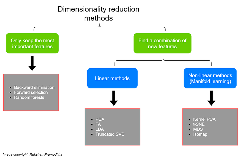
High Dimension Data Analysis - A tutorial and review for Dimensionality Reduction Techniques
High Dimension Data Analysis - A tutorial and review for Dimensionality Reduction Techniques
This article explains and provides a comparative study of a few techniques for dimensionality reduction. It dives into the mathematical explanation of several feature selection and feature transformation techniques, while also providing the algorithmic representation and implementation of some other techniques. Lastly, it also provides a very brief review of various other works done in this space.