Reconfigurable Computing Course Associated with the Long Short-Term Memory and the High-Level-Synthesize

Abstract

Long short-term memory(LSTM)is a periodic neural network that is suitable for predicting and processing time series intervals and relatively long-delayed important events. In this paper, there are five Lab about the basic principles of LSTM and the methods of generating IP core in the Vivado HLS that has been finished. In addition, the results are confirmed on Zedboard. This experimental course help us understand the principle of LSTM and acquire the skills of cooperative development of ARM and FPGA.

Index Terms - LSTM, Reconfigurable Computing, HLS, Vivado

1. Introduction

2. A. Long short-term memory

Long short-term memory (LSTM) units are units of a recurrent neural network (

R N N)

. An RNN composed of LSTM units is often called an LSTM network. A common LSTM unit is composed of a cell, an input gate, an output gate and a forget gate. The cell remembers values over arbitrary time intervals and the three gates regulate the flow of information into and out of the cell.

LSTM was proposed in 1997 by Sepp Hochreiter and Jürgen Schmidhuber and improved in 2000 by Felix Gers' team [1] [2]. Nowadays, LSTM has been applied in the fields of science and technology.A time series prediction model was proposed based on combination of the longshort time memory neural network model and the Dynamic Bayesian Network (DBN) by Qinkun Xiao in 2017 [3], and in 2018 LSTM was used in a bipedal robot by Christos Kouppas [4]. Otherwise, applications of LSTM also include: music composition [5], grammar learning [6], predicting subcellular localization of proteins

[7]

and etc.

The most widely used LSTM network is currently using the LSTM unit in Fig. 1 instead of the RNN network of the original RNN implicit layer. The LSTM unit is specifically designed with memory units for saving historical information. The update and use of historical

Fig. 1. conveyer belt structure.

information are controlled by three doors, one by one entry door, forgetting door, output door. Fig. 1 shows a the conveyer belt structure of LSTM block with input, output, and forget gates. There are many other kinds of LSTMs as well.

3. B. High-level synthesized

Early academic work extracted scheduling, allocation, and binding as the basic steps for high-level-synthesis. Scheduling partitions the algorithm in control steps that are used to define the states in the finite-state machine. Each control step contains one small section of the algorithm that can be performed in a single clock cycle in the hardware. Allocation and binding maps the instructions and variables to the hardware components, multiplexers, registers and wires of the data path.

First generation behavioral synthesis was introduced by Synopsys in 1994 as Behavioral Compiler and used Verilog or VHDL as input languages. The abstraction level used was partially timed (clocked) processes. Tools based on behavioral Verilog or VHDL were not widely adopted in part because neither languages nor the partially timed abstraction were well suited to modeling behavior at a high level. 10 years later, in early 2004 , Synopsys end-oflifed Behavioral Compiler.

In 2004 , there emerged a number of next generation commercial high-level synthesis products (also called be- havioral synthesis or algorithmic synthesis at the time) which provided synthesis of circuits specified at

C

level to a register transfer level (RTL) specification. Synthesizing from the popular

C

language offered accrued abstraction, expressive power and coding flexibility while tying with existing flows and legacy models. This language shift, combined with other technical advances was a key enabler for successful industrial usage. High-level synthesis tools are used for complex ASIC and FPGA design.

High-level synthesis (HLS) was primarily adopted in Japan and Europe in the early years. As of late 2008 , there was an emerging adoption in the United States.

HLS, proposed by an American company , sometimes referred to as

C

synthesis, electronic system-level (ESL) synthesis, algorithmic synthesis, or behavioral synthesis, is an automated design process that interprets an algorithmic description of a desired behavior and creates digital hardware that implements that behavior. Synthesis begins with a high-level specification of the problem, where behavior is generally decoupled from e.g. clocklevel timing. Early HLS explored a variety of input specification languages. Although recent research and commercial applications generally accept synthesizable subsets of ANSI C/C

+ + /

SystemC/MATLAB. The code is analyzed, architecturally constrained, and scheduled to transcompile into a register-transfer level (RTL) design in a hardware description language (HDL), which is in turn commonly synthesized to the gate level by the use of a logic synthesis tool.

Hardware design can be created at a variety of levels of abstraction. The commonly used levels of abstraction are gate level, register-transfer level (RTL), and algorithmic level.

4. Contents of the LSTM Network Experiment

5. A. Lab 1 - Familiarlisation and Testbench

The purpose of this section is to help us understand the principle of LSTM. In the xsimple.py program, there are four major paraneters including length of vectors, length of output predictions, batch size and sequence length. Find and change these four paraneters and change the source code so the file containing main() (which we will call the testbench ) and the

lstm ()

function are in separate files. Otherwise, the MAXERR, MSE and AMSE can be also calculated by the program that I have changed before.

6. B. Lab 2 - Parallelism

The purpose of Lab 2 is to gain our experience in optimising a design with compiler directives in Vivado HLS. This Lab can be devided in two parts: part one is to create a Vivado HLS project and part two is to explore how compiler directives such as LATENCY, DATAFLOW, ARRAY PARTITION, UNROLL and PIPELINE can improve the speed of the design. The descriptions of such five directives are shown below. a) LATENCY: The latency of the design is the number of cycle it takes to output the result. Fig. 2 shows the example of 10 cycles design LATENCY.

Fig. 2. 10 cycles design LATENCY.

b) DATAFLOW: Enables task level pipeline, allowing functions and loops to execute concurrently. Used to minimize interval.

c) ARRAY PARTITION: Partitions large arrays into multiple smaller arrays or into individual registers, to improve access to data and remove block RAM bottlenecks.

d) UNROLL: A standard loop of

N

iterations can be unrolled to by a factor. Fig. 3 shows the UNROLL operation and result. It seems that Unrolled loops are likely to result in more hardware resources and higher area.

Fig. 3. The UNROLL operation and result.

e) PIPELINE: Pipeline allows operations to happen concurrently. The task does not have to complete all operations before it begin the next operation. Pipeline is applied to functions and loops. Fig. 4 shows the comparision between the function with and without piplining.

Fig. 4. The comparision between the function with and without piplining.

In addition, the performance of modification can be evaluated by four parameters including number of cycles

T

, area

A

(defined as the percentage of the most used resource out of LUTs, memories and DSPs) and AT product.

7. Lab 3 - Precision

Fixed-point arithmetic requires less area and has lower latency than floating-point. Moreover, FPGAs can more efficiently perform low-precision calculations than processors and graphics processing units. The Vivado HLS ap_fixed type is used to modify the floating-point implementation. Then synthesize the design using HLS and run the

C

simulation to verify the output.

In Vivado HLS, it is important to use fixed-point data types, because the

C + +

/ System C simulation performed using fixed-point data types matches the hardware created by the synthesize. This enables you to analyze the impact of bit precision, quantization, and overflow with fast c level simulation. It can be seen from the experimental results that when the fixed point data type is used, the delay will be greatly reduced.

8. Lab 4 - Exploration

In this experiment we explore how to obtain the maximum speed in our LSTM implementation. We can apply any optimisations as long as the the percentage error for any output (compared with the original double precision

C

version) is less than

10 %

. Various methods has been adopted such as the

C

source code modification, approximations introduction, trying different fixed point rounding modes and changing directives, in order to achieve the minimum number of cycles for the LSTM implementation at

100 M H z

. Otherwise, the execution time

(T \times p)

has been optimised where

p

is the clock period, by setting tighter timing constraints.

9. E. Lab 5 - Interface

In this lab, a Zynq design for the xc7z020clg484-1 FPGA is needed to create on the Zedboard with the LSTM design included as an IP Block. The performance of the accelerated design is compared to the pure Zynq implementation and the original desktop implementation. Improve the performance of accelerated design using software or hardware technology. Ideas include:

Find better ways to calculate nonlinearities;
Reducing precision requirements;
Before rounding, the accumulation of higher accuracy;
Improve the design clock frequency.

10. Operations and Results

A. Modifications of LSTM Python Code and C

+ +

Code

Fig. 5 shows the code, including the MAXERR, MSE and AMSE calculation function, that I add in main.cpp file. In addition, the calculation results are also shown in

Fig. 5. The calculation code that I added and The calculation results.

11. B. Add Pipeline Directly

Add simple.cpp to HLS project, click on Run C to synthesize toolbar button. When the synthesize is complete, the report file opens automatically. The result is shown in Fig.

6 .

\begin{array}{rrrr} Clock & Target & Estimated & Uncertainty \\ ap_clk & 10.00 & 9.78 & 1.00 \end{array}

Latency (clock cycles)

Fig. 6. The comparision between the function with and without piplining.

12. Add Interface

As shown in Fig. 7, the interface for the input and output variables, mode select axilite have been added.

13. - Istm

% HLS INTERFACE s_axilite register port=return % HLS PIPELINE

% HLS INTERFACE s_axilite register depth

= 4

port=h -

x

14. $%$ HLS INTERFACE s_axilite register depth $= 4$ port=x

Fig. 7. The comparision between the function with and without piplining. Fig. 5 . D. Creat an IP Core

Click on the Run C synthesize toolbar button, and the final step of the advanced synthesize process is to package the design as an IP block for other tools in the Vivado design suite. Click the Export RTL toolbar button. The IP wrapper creates a package for the Vivado IP directory. E. Create a Vivado Project

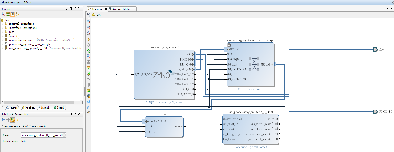
Create a vivado design suite project, create a block design and add HLS IP to block design. Xilinx IP block LSTM is now instantiated in the design. Then add Zynq7 processing system to the block design. The design block now has two IP blocks. The next step is to connect HLS blocks to the Zynq block and ports. The block design is shown in Fig. 8 The more specific operations are as follows.

Fig. 9. the icon of SDK.

Learn to optimise a design with compiler directives

in Vivado HLS;

Know the design process in converting floating-point designs to fixed-point;
Quantify the performance advantages of fixed-point over floating point for our long short-term memory (LSTM) example;
Acquire the skills of cooperative development of ARM

Fig. 8. Connect HLS IP core to the ZYNQ7 processing system. and FPGA.

F. Debug Hardware in PL and Software in PS

The hardware debug operations after finishing the block design are shown below:

Click Generate Bitstream to initiate the remainder of the flow:
From the Vivado File menu select Export $>$ Export Hardware. In the Export Hardware dialog box ensure that the Include Bitstream is enabled and click OK;
From the Vivado File menu, select Launch SDK. Select New $>$ Application Project;

Then we can see the icon of SDK shown in Fig. 9 and drive HLS IP in Helloworld.c. We should initialize the HLS IP. The software debug operations are shown below:

Power up the ZedBoard and test the Helloworld.c application. Ensure the board has all the connections to allow you to download the bitstream on the FPGA device. See the documentation that accompanies the ZedBoard development board;
Click Xilinx Tools > Program FPGA (or toolbar icon). Notice that the Done LED (DS3) is now on;
Click Run As > Debug on Hardware.

15. Conclution

In addition, with the help of teachers and classmates, a lot of problems that I met with had been solved. I have learned a lot and I am very grateful to my teachers and classmates for their help.

16. References

[1] S. Hochreiter and J. Schmidhuber, "Long short-term memory," Neural Computation, vol. 9, no. 8, pp. 1735-1780,

1997 .

[2] F. A. Gers, J. Schmidhuber, and F. Cummins, "Learning to forget: continual prediction with 1stm," in International Conference on Artificial Neural Networks ICANN, 2002, pp. 850-855.

[3] Y. S. Qinkun Xiao, "Time series prediction using graph model," in 2017 3rd IEEE International Conference on Computer and Communications (ICCC). IEEE, 2017, pp. 1358 - 1361 .

[4] C. Kouppas, "Machine learning comparison for step decision making of a bipedal robot," in 2018 3rd International Conference on Control and Robotics Engineering (ICCRE). IEEE, 2018, pp. 0-4.

[5] D. Eck and J. Schmidhuber, "Learning the long-term structure of the blues." Lecture Notes in Computer Science, vol. 2415, pp. 284-289, 2002.

[6] J. A. Pérezortiz, F. A. Gers, D. Eck, and J. Schmidhuber, "Kalman filters improve lstm network performance in problems unsolvable by traditional recurrent nets." Neural Networks the Official Journal of the International Neural Network Society, vol. 16, no. 2, pp.

241 - 250, 2003 .

[7] T. Thireou and M. Reczko, "Bidirectional long short-term memory networks for predicting the subcellular localization of eukaryotic proteins," IEEE/ACM Transactions on Computational Biology and Bioinformatics (TCBB), vol. 4, no. 3, pp. 441-446,

2007 .