Divide-and-conquer sort: heap sort

1. heap

Heapsort is a comparison-based sorting algorithm in the field of computer, which can be regarded as an optimized implementation of selection sorting. The similarity between heap sort and selection sort is that the input array is also divided into sorted and sorted regions, and the operation of extracting the maximum value from sorted region and inserting it into sorted region is repeatedly performed, so as to continuously reduce sorted region.The difference between them lies in the way to obtain the maximum value of the sorted area. Heap sort does not waste time on linear scanning of the sorted area, but keeps the structure of the heap and only needs to complete the repair operation of the heap each time, thus greatly reducing the time to obtain the maximum value in each step^[1].

2. The definition of the heap

consider the following two question.

Why is the structure of the heap defined this way? What are the benefits?
In the process of heap design, heap implementation and heap analysis, it is because of the structure characteristic or partial sequence characteristic of heap that the process can be smoothly advanced.

A binary tree is defined as a heap if it satisfies both heap structural properties and heap partial ordering properties:

The heap structure properties are that a binary tree is either perfect, or it has only a few fewer nodes in the bottom layer than a perfect binary tree, and the bottom nodes are placed next to each other from left to right.
The heap partial ordering property means that the heap node stores elements such that the value of the parent node is greater than the value of all the children (the size relationship between the left and right child nodes is not required).

3. Abstract maintenance of the heap

3.1 Heap of repair

According to the partial order characteristic of heap, the largest element must be located at the top of heap, which makes heap widely used in sorting, priority queue and other occasions. So we need to fix it efficiently once the largest element at the root of the heap is removed to make it a heap again.

The process of heap repair is essentially the process of heap structural characteristics and heap partial order characteristics repair

For structural features, there is a vacancy, so it needs to be filled in.
For partial ordering, the left and right subtrees of the heap are still a legal heap, even though the top element is removed.

The two properties are orthogonal, which allows us to focus on fixing structural properties first, and fixing partial order properties later.

The repair of sstructure properties is very simple due to the special nature of the heap structure: since the elements at the bottom of the heap need to be arranged from left to right, we can "safely" remove the bottom right-most elements without damaging the heap structure. So the fix to the heap structure is to take the bottom rightmost element and put it at the top of the heap.
For the repair of partial order property, we are faced with a binary tree that meets the heap structure property. Its left and right subtrees are legitimate heaps, but its root node does not meet partial order property between the left and right child nodes. To this end, we do the following:
- Compares the values of the parent node with those of the two children. Swap the larger value of the two child nodes (let's say the left node) with the parent.
- As a result of the above operation, we introduce a new root node for the left subtree, which may violate partial order, so we need to recursively repair the left subtree as described above.

Since heaps are repaired only on a strictly decreasing series of subtrees at height, the number of repairs must not exceed the height of the heap. Because of the heap structure, its height is

O (\log n)

, and the number of comparisons for each repair is

2

, i.e. the time complexity of

O (1)

(which can be optimized), so the cost of heap repair is

O (\log n)

3.2 Heap construction: floating up

The float up process only requires $1$ comparisons with the parent node

The heap construction process can be thought of as inserting

N

elements to be sorted into the binary heap. Since each operation requires an up-float operation (the number of times is the depth of the node)

https://spectra-images-production.s3.amazonaws.com/articles/2022.04.00067/dcde92b1-cca8-44ef-8fd8-a4ff0b281409.png

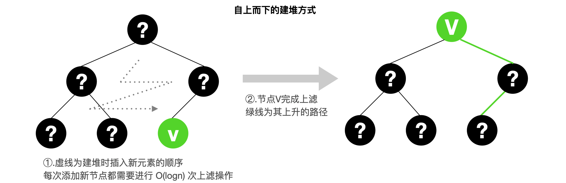
For a perfect binary tree, the points whose depth is

h

are

2^{h}

, then the total time complexity is:

\begin{aligned} W (n) & = \sum_{h = 0}^{⌊ \log n ⌋} 2^{h} O (h) \\ = \sum_{h = 0}^{⌊ \log n ⌋} h \cdot 2^{h} \\ = (2 ⌊ \log n ⌋ - 1) 2^{⌊ \log n ⌋} + 2 \\ = O (n \log n) \end{aligned}

Although the time complexity of this heap construction is not as low as

F l o y d h e a p

construction, the floating operation in binary heap can optimize the heap repair process in heap sorting!

3.3 Heap construction: sinking

The sinking process requires a $2$ comparison with the left and right child nodes

3.3.1 Algorithm implementation

It is easy to maintain a set of nodes as a binary tree that satisfies the heap structure characteristics (see discussion in 3)^[2]. Suppose we have a binary tree that satisfies the heap structure, but the size relationship between the values stored by each node in the tree is chaotic. Now we need to satisfy the heap partial order between all the parent nodes in the tree. Based on the repair operation of the heap in 2.1, it is easy to construct the heap by recursion:

Build the heap from the root.
For the left and right subtrees of the heap structure, it is only necessary to recursively build them all into a valid heap first.

3.3.2 algorithm analysis

We can briefly analyze the complexity of heap builds based on the analysis of heap repair operations. The worst-case time complexity of sequential heap repair is

O (\log n)

, which requires at most one repair operation for

N

elements, so the heap construction cost is

O (n \log n)

. But this analysis is very crude!

The recursive algorithm is described by the recursive equation, and the cost of the recursive algorithm is obtained by solving the recursive equation

We analyze algorithm2 and obtain the following recursion

W (n) = 2 W (\frac{n}{2}) + 2 \log n

according to the

M A S T E R

theorem, there exsit

ε > 0

satify

\log n = O (n^{1 - ε})

, so

W (n) = O (n)

This conclusion is inconsistent with the

O (n \log n)

obtained above, because the worst-case time complexity of heap repair is

O (\log n)

, which is a very loose estimate. Strictly speaking, a node heap repair costs no more than

2 h

, where

H

is the height of the node. And the number of nodes whose height is

h

for a perfect binary tree is

⌈ \frac{n}{2^{h + 1}} ⌉

^[3].

Therefore, for a perfect binary tree, we just need to count the cost of nodes at each layer and sum up to get the total heap repair cost:

\begin{aligned} W (n) & = \sum_{h = 0}^{⌊ \log n ⌋} ⌈ \frac{n}{2^{h + 1}} ⌉ O (h) \\ = O (n \sum_{h = 0}^{⌊ \log n ⌋} \frac{h}{2^{h}}) \\ = O (n) \end{aligned}

4. Concrete implementation of heap (Data structure Design)

To implement a heap, the natural place to start is with the definition of a heap. The definition of a heap has two orthogonal properties: structure property and partial order property. The partial order property is intuitively more important because it makes it easier to find the largest element. To this end, should we use a linked list structure where both parent and child nodes can access each other through Pointers? This implementation is fine for the partial ordering nature of the heap, but the main problem is that it is not easy and efficient to take an element from the bottom right for heap repair, which is very important for heap structure maintenance.

So what structures can easily maintain the structural characteristics of the heap? Let's look at another key operation, how to quickly and easily implement the parent-child node relationship?

We can place elements in a binary tree in an array in descending order of depth, and elements of the same depth from left to right.

We can identify the following mathematical properties:

$PARENT$ ( $i$ ) = $⌊ \frac{i}{2} ⌋$
$LEFT$ ( $i$ ) = $2 i$
$RIGHT$ ( $i$ ) = $2 i$ + $1$

The above three properties can be rigorously proved mathematically.

E [I]

is the th

k

element of the

j

layer, so

i = (2^{j - 1} - 1) + k

Then the serial number of its left child node is

i + (2^{j - 1} - k) + 2 (k - 1) + 1 = 2 i

Based on the array implementation of the heap, we can implement the repair and build operations of the heap discussed earlier.

5. summary

With the partial ordering guaranteed by the heap, it's easy to use it for sorting. The heapsort algorithm first builds all the elements into a heap. Based on the heap, the algorithm can immediately get the global largest element. Remove the largest element and place it at the end of the output sequence. For the heap with the root node removed, the algorithm performs heap repair. By repeating "root and fix" above, we can sort all the elements. The cost of building the input

n

elements into a heap is

O (n)

, and the cost of each heap repair is

O (\log n)

, so the worst-case time complexity of heap sort is

O (n + n \log n) = O (n \log n)

. According to the discussion on the lower bounds of the worst case and average case time complexity of comparison sort, we know that the worst case time complexity of heap sort reaches the optimal of comparison sort. Meanwhile, the average case time complexity of heap sort is also

O (n \log n)

, which also reaches the optimal value.

6. Optimization direction

Through the worst-case time complexity analysis of heap sort, we can know that the process of "root and repair" is the key step that affects the time complexity. The repair process is the sink process of the root node, which requires a

2

comparison with the left and right child nodes^[4].

\begin{aligned} W (n) & = \sum_{h = 0}^{⌊ \log n ⌋} 2^{h} O (h) \\ = \sum_{h = 0}^{⌊ \log n ⌋} 2 h \cdot 2^{h} \\ = (2 ⌊ \log n ⌋ - 1) 2^{⌊ \log n ⌋ + 1} + 4 \\ = O (n \log n) \end{aligned}

There is a "fact" that the "roots" taken from the bottom of the heap tend to be small, meaning that the heap can be repaired by swapping places with the larger values of the left and right child nodes. And this sinking process only requires

1

comparison! We call it Risky Sink

The "Risky" means that the node excessively sinks, resulting in a larger situation than its parent; in this case, a landing operation is required (again, only one comparison is required).

Here we can use the idea of binary search, sink to half depth, check whether the heap partial order characteristics are satisfied, if so, then sink to

\frac{1}{4}

depth, check whether the heap partial order characteristics are satisfied, and repeat. If the partial order is not met, float up until the partial order is met.

7. generalization

By the extension of binary heap, we can get the definition of

d

binary heap (including structural characteristics and partial order characteristics). At the same time, we can obtain the mathematical relation of the serial number of the parent node in

d

fork heap (see problem 5.3), just like the mathematical relation of the serial number of the parent node in the binary heap^[5].

We can observe the difference between binary heap and

D

heap: height and width

Binary Heap (thin and tall)
- height： $\log_{2} n$
- width： $2$
$D$ $D$ DD $D$ Heap (chunky)
- height： $\log_{d} n$
- width： $d$

Whether binary heap or

d

heap, can do the sorting operation. But they have different costs in the process of rising and sinking

Float up: the child node only needs to compare $1$ with the parent node, and is independent of the number of children. The total cost is about $O (\log_{d} n)$ , so the lower the better
Sink operation: parent nodes need to be compared $d$ times with $d$ child nodes, the total cost is about $O (d \log_{d} n)$ , so the thinner the better

Reference

Cormen T H, Leiserson C E, Rivest R L, et al. Introduction to algorithms[M]. MIT press, 2022. ↩︎
Schaffer R, Sedgewick R. The analysis of heapsort[J]. Journal of Algorithms, 1993, 15(1): 76-100. ↩︎
Wegener I. Bottom-up-heap sort, a new variant of heap sort beating on average quick sort (if n is not very small)[C]//International Symposium on Mathematical Foundations of Computer Science. Springer, Berlin, Heidelberg, 1990: 516-522. ↩︎
Carlsson S. A variant of heapsort with almost optimal number of comparisons[J]. Information Processing Letters, 1987, 24(4): 247-250. ↩︎
Jung H. The d-deap*: A fast and simple cache-aligned d-ary deap[J]. Information processing letters, 2005, 93(2): 63-67. ↩︎

Heap sort