J. Whinnery, W. Buchanan, A. Kumar, H. Ly, B. Swidenbank, D. Winek, A. Yuen

University of California at Berkeley, December 10, 2021

Introduction

The purpose of this project was to design a system involving a test impact table that utilizes low-cost piezoelectric vibration sensors in conjunction with custom trilateration algorithms and signal processing to pinpoint the location of impact. A piezoelectric sensor is a device that uses the piezoelectric effect to measure changes in pressure, acceleration, temperature, strain, or force by converting them to an electrical charge [1]. The motivation behind this project was derived from the uses of impact detection and its applications towards important practices such as manufacturing and maintenance. A classical example determining location involves triangulation (e.g: GPS), wherein a device encodes a timestamp and bounces a signal off three satellites, using the time traveled to each of the satellites and the speed of sound to find the source location. In the project, the time of impact is not a known quantity; as such, the team developed different tests and algorithms characterizing location. Initially, it was decided to use piezoelectric vibration sensors guided by a custom-built DAQ (Fig. 1b) and a mechanical dropper system in an attempt to accurately characterize impact locations.

For initial characterization of the data to determine impact location, the team developed two algorithms in parallel. The magnitude based approach was developed with the assumption that the magnitude output from the sensor would be consistent and inversely proportional to the distance from the point of impact. The consideration of propagation time followed in the same vein; the group’s hypothesis was as follows: the further the impact from the sensor, the longer it would take the sensor to register the effects of vibration. Some assumptions the group made included that the speed of propagation across the impact material is constant and mirrors the speed of sound in that material. From these assumptions, both magnitude and time based algorithms were created to determine impact location based on collected data.

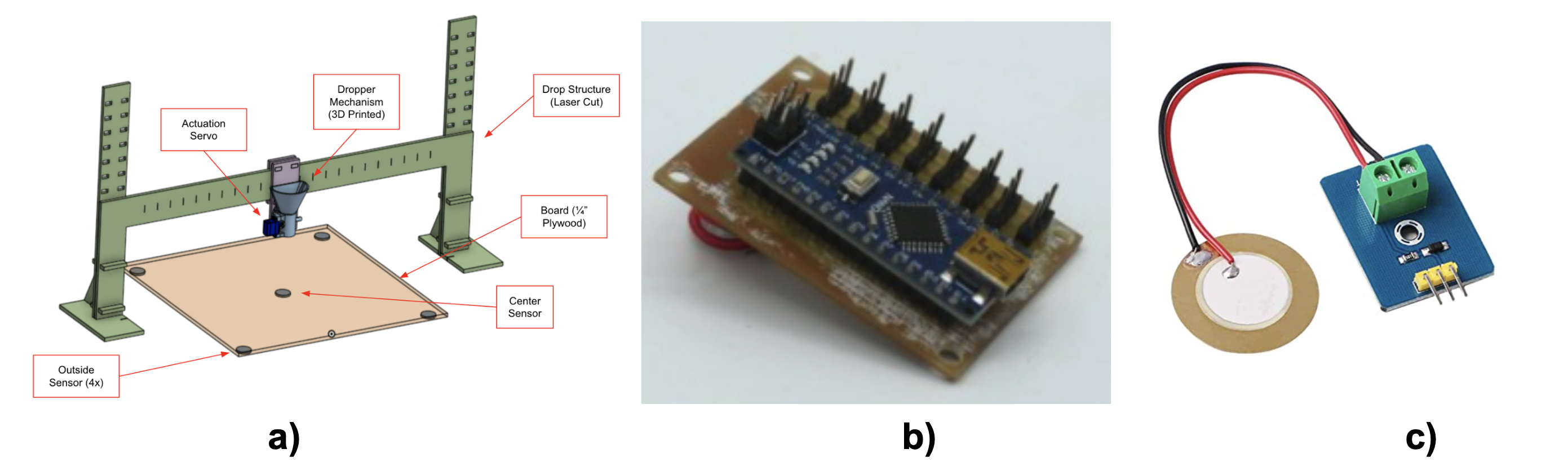The team believes the findings can apply to industrial applications including aerospace maintenance (accurate bearing life tracking), hail damage (localized damage detection), CNC maintenance (tooling life indicator), and military/defense (impact detection). Figure 1. a) Mechanical system coupled with multiple sensors on test table grid b) Custom PCB for DAQ c) Inexpensive piezoelectric sensor and amplifier

Methods

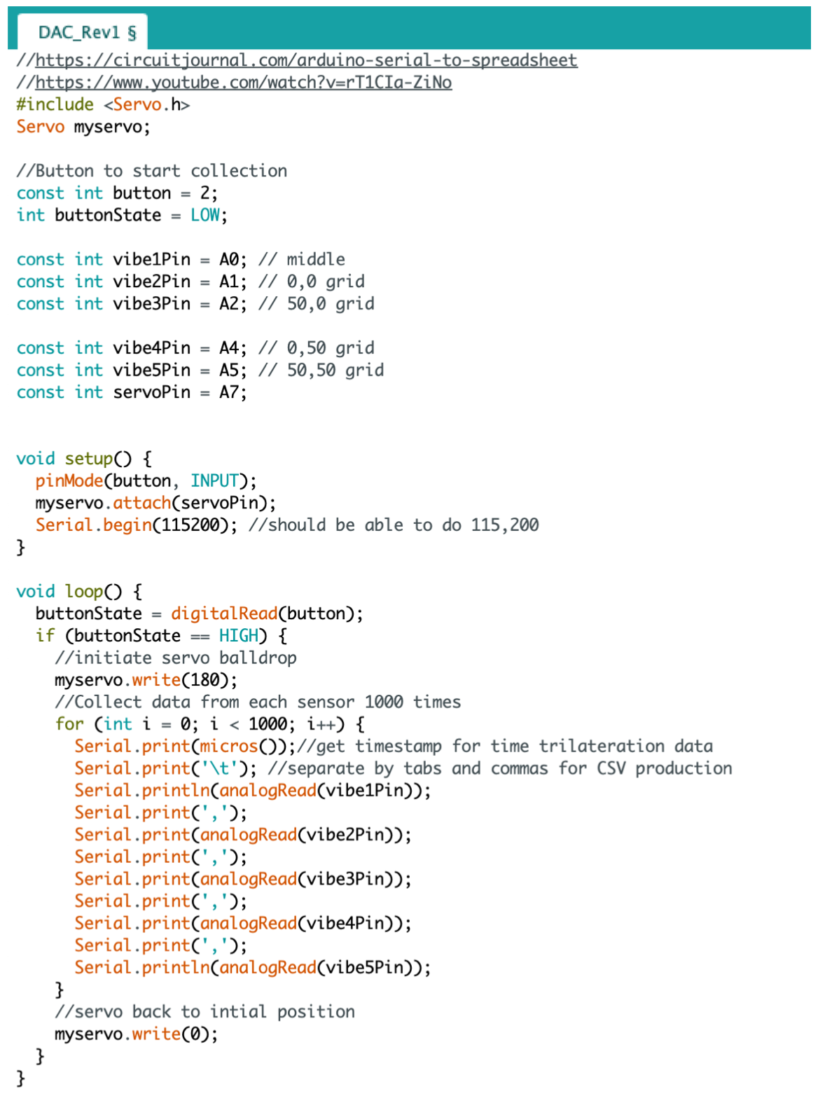
A 2’ x 2 ’x 0.25” piece of plywood was laser cut with a centimeter grid laser etched onto the surface. To get a finer resolution, the team decided to attach five sensors (as opposed to the three needed for trilateration) at measured locations on the board. The corner sensors were not placed exactly on the corner of the board (Fig. 1a) to eliminate vibration attenuation that can occur along the edge of the board. In addition to the board, the team designed a custom automated ball dropper mechanism and fixtures to ensure a consistent drop height and location. With the test setup and hardware, a metal ball was dropped onto 50 different locations on the grid. In order to record the location of the drop, a team member would visually observe the ball landing site and record the corresponding grid number. Data was collected using an Arduino Nano and custom PCB manufactured in-house (for convenience and organization). Each piezo sensor connects through an amplifier to alternating analog pins (to mitigate noise) of the Arduino. Through the built-in analogread() function and a custom Arduino IDE [4], a button push triggers the collection of 1000 data points from each of the 5 sensors (Appendix A).

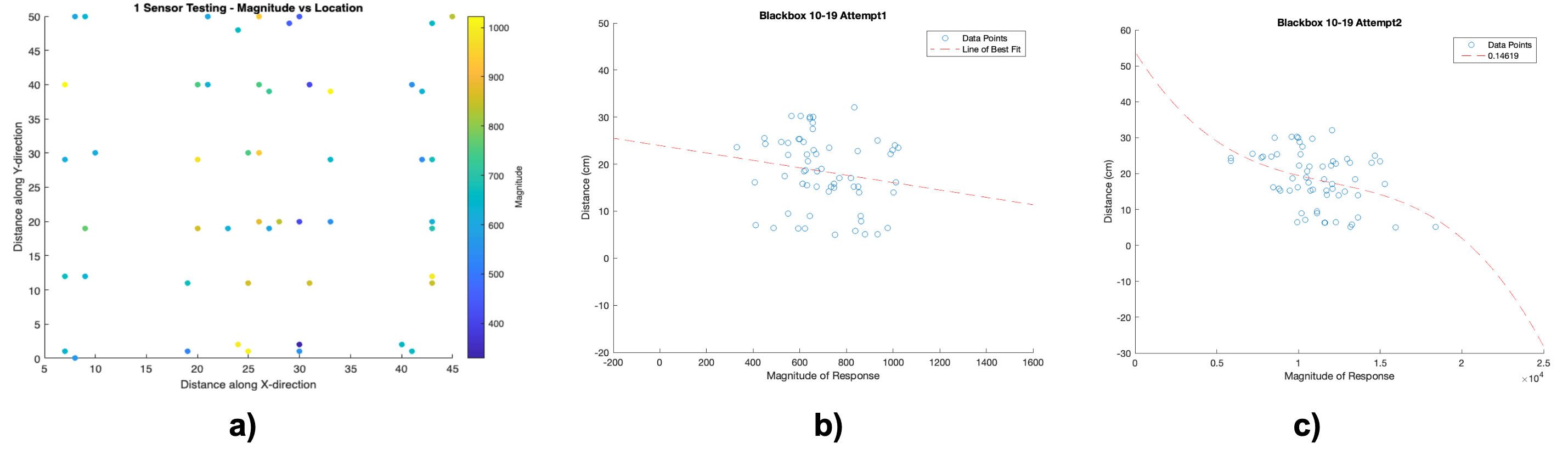
Figure 2. a) Center sensor magnitudes vs. drop locations showing no trend b) Blackbox linear fit with R2 = 0.09 c) Improved blackbox cubic fit with R2 = 0.14

As shown in Fig. 2, initial characterization attempts using the peak magnitude values yielded a 0.09 R2 value indicating a virtually random distribution. In an attempt to average out the poor sampling frequency and accounting for the shape of the response, the team blackboxed the data using the peak value summed with a few additional values after it. While this improved the R2 value from 0.09 to 0.14, the correlation remains poor. When initially determining the feasibility of using piezoelectric sensors for trilateration, the team also considered the uncertainty of the sensor outputs in addition to calculating the correlation between sensor output and distance.

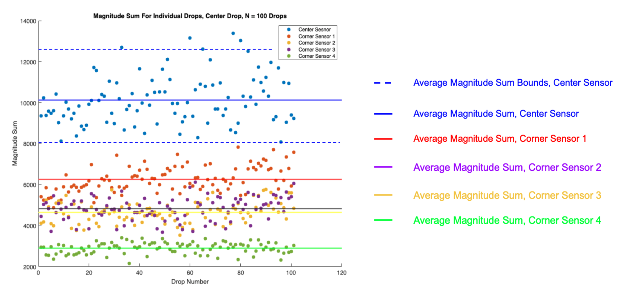
Figure 3. Magnitude sums and their averages of each sensor across 100 center drops

The team proceeded to perform an experiment where 100 metal ball drops were repeated directly over the center of the board. Ideally, to determine the bias error of the sensors, the sensor specification data sheet provided by the manufacturer would have a precision specification. Unfortunately, the team was unable to acquire the data sheet as piezoelectric sensors are not necessarily precision measurement devices. The team then created a custom method to determine bias error of the system, using the magnitude sum distributions for the four corner sensors. The magnitude sum is the sum of all measured magnitude values of a bounce, as this better quantifies the energy of a ball drop than would taking the peak magnitude of a bounce. Theoretically, the 4 corner sensors should have identical means for a drop in the center of the board but that was not the case (Fig. 3). This variation in mean values is considered to be the systematic error, forming in aggregate from differences in sensor attachment, material anisotropy, and relative drop location.

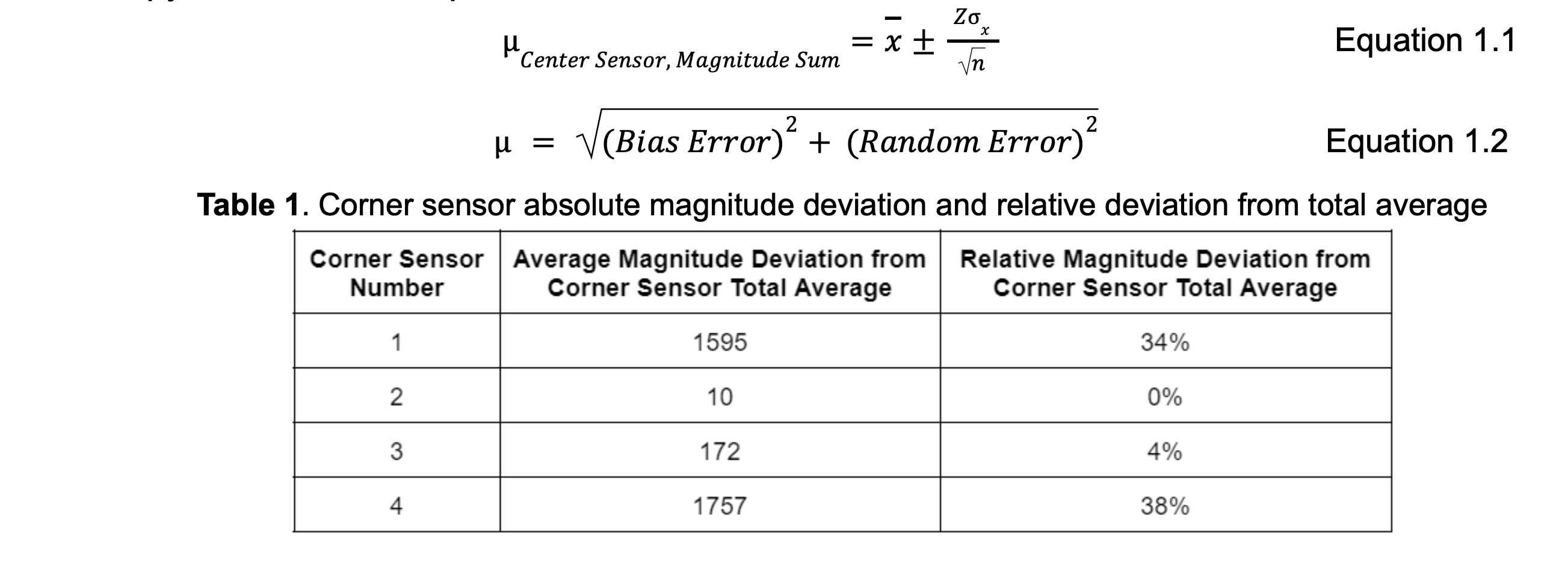
To determine the systematic error, the average of all data points for the four corner sensors was computed, as well as the averages for the individual corner sensor magnitude sum distributions. From Table 1, Corner Sensor 4 had the largest variation from the overall average of corner sensor magnitude sums, so that is the assumed systematic error. Based on the spread of the magnitude sum distribution, the center sensor had the largest variation relative to the other sensors, so the data for the center sensor was used to calculate the relative random error, using a Z of 95% confidence interval. The spread for the center sensor is largest because it is closest to the ball drop position, and with impact energies close to sensor saturation, non-linearities in the sensor will create large random variations. Using Equation 1.1, the true average value of the magnitude reading of the center sensor will fall within 10128 ± 231. With this interval, the relative random error is ± 2%.

With the relative bias and random errors, Equation 1.2 is used to find the uncertainty of the magnitude sum measurement, which was ± 38%. With this high uncertainty calculation coupled with the poor correlation between magnitude and distance, the team decided to drive a different approach to the problem: determine the height an object was dropped from and validate the sensors in a simpler use case. As the height of the ball is directly proportional to its impact load, and only one sensor is used (with the full load of the ball going through it rather than vibrations washing over it), this should help to isolate sensor issues and further characterize the sensors to see if consistent data can be taken.

For the 1D distance to impact characterization, the team decided to initially test a load cell sensor due to the familiarity with the sensor’s load response and the presence of available datasheets for the sensor. This sub-experiment was designed to also act as a source of comparison and validation for the piezoelectric sensors. The team designed and manufactured a test fixture which would enable consistent drops at desired heights onto the sensor. This test fixture consisted of a 3D printed ball dropper and a sensor housing. The ball dropper was a hollow cylindrical part with a three-point guide system internally which was designed to ensure the ball impacts the same location for every drop (Fig. 4a). A thin piece of wood was inserted through the slots of the dropper which made up the dropper system for the ball. For the purpose of the test, during sampling, the wood was manually pulled out and the ball, in turn, was dropped from the desired height. The housing was designed in a manner that it clamped the load cell down to a cantilever position. A 3D printed surface was mounted onto the impact end of the load cell to ensure a dampened and smoother transfer of momentum and energy from the ball to the strain gauge. Data was collected from 3.67” to 12.67” in increments of 1” by dropping a rubber ball from these heights onto the load cell. Rubber balls were used as they fit within the specifications of load for the sensor- accounting for height- and to increase the impact time. A total of 20 tests were performed at each position with a sampling rate of 80Hz limited by the use of the HX711 amplifier for the load cell used.

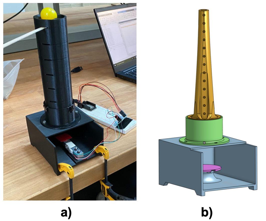
Figure 4. a) Ball drop fixture for load cell b) BB drop fixture for piezo sensor

The max load cell output for each test was determined and the average max output for a particular height position was calculated. This was then compared to the height of the drop. As expected, while analyzing the data from these tests, the load cell output is directly proportional to the height of drop but there were several inconsistencies. One of the key concerns was that due to repeated impact of the rubber onto the load cell for different height positions, there was an effect of creep acting onto the outputs. Studying the load cell data sheet it was decided that the best way to account for creep was to use the difference between the max output value and average of the no load values i.e to purely use the amplitude of the load cell output curve. An improvement in the trend was noticed (Fig. 5). According to the specification sheet, the change in resistance, which is essentially what the load cell output produces, is linearly proportional to load/weight. Based on conservation of linear momentum and energy it is known that load varies linearly with height. Hence, a linear fit was implemented to the data and the team was able to achieve an R2 value of 0.66, a significant improvement compared to previous measurements. The total bias error of the system was calculated using the error bound of the curve fitting. The bias error here takes into account improper calibration and consistent inaccuracies produced by the test fixture setup. The total precision error of the system was determined through the use of the t-distribution table since the number of samples per test location was less than 30. A 95% confidence interval was used to carry out these calculations. As a result, the system has a total relative error of ±10.89%. Hence, from this sub-experiment the team was able to identify key areas of improvement when it comes to sensor magnitude data analysis; the use of a rubber ball enabled a better differential between data at different height locations from a greater impact time corresponding to a relatively higher sampling frequency.

Figure 5. a) Load cell output at height = 8.67” b) Linear fit of plot representing avg magnitude vs height for the load cell height characterization

In parallel with the load cell testing fixture, a 1D piezo sensor test stand was developed in order to isolate and reduce sensor inconsistencies. One way that inconsistency was mitigated was via a 3D printed fixture with an area for soldered sensor leads to come out, allowing the sensor to lay flat on the drop board and also attach flatly to the surrounding box. Through use of only a single sensor, as opposed to five, sampling frequency saw a roughly 3X speedup as well. As rubber balls proved to be too heavy with all the load going through the sensor, airsoft pellets (0.2 g) were used as a replacement. For this, a new fixture was created to accurately drop the drastically smaller balls. The first iteration had too much resistance (high frequency of impact with walls upon exit) and resulted in a significant delay in the ball falling. This was problematic as it introduces inconsistency and degrades the relationship between drop height and potential energy. To fix this, the hole was widened, and draft angle added along with reduction to only three points of contact for guiding the ball down the chamber. Additionally, VHB tape attached the sensor to the drop platform and box to eliminate inconsistent compression using painter’s tape. Data was collected at a starting height of 3.5 inches, with height increasing by 1 inch every 10 data points on the x-axis. From data analysis, it was also noticed that utilizing the calibrated sum of the magnitudes produced better results as compared to the max magnitudes as there is a significant reduction in standard deviation. There appear to be two groupings of data (Fig. 6a), one with low recorded values, and one with the expected logarithmic growth trend (as height increases, so do collisions with walls on the way down the chamber, decreasing velocity and effective height dropped from - air resistance also has a relatively high impact on light objects).

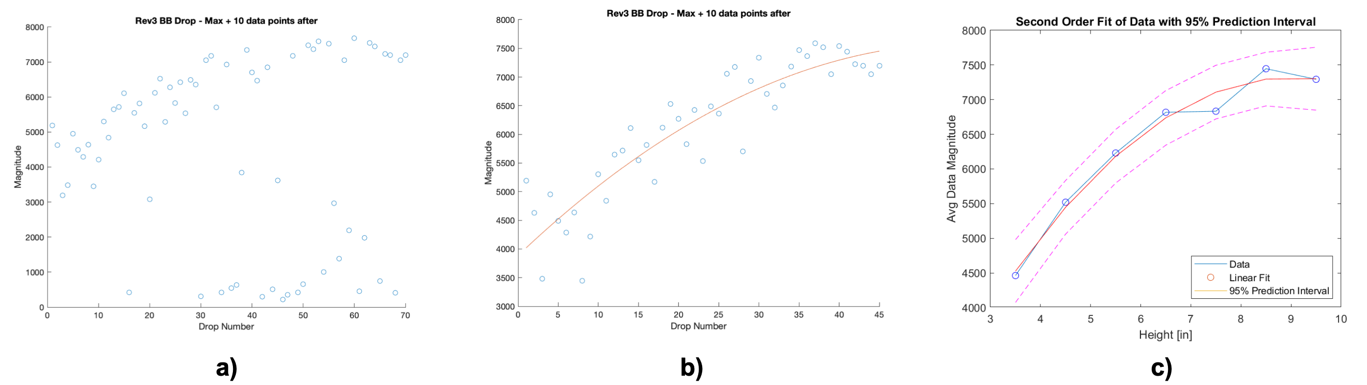
Figure 6. a) Raw magnitude vs drop number for height characterization b) Magnitude vs drop number with outliers removed and trendline shown c) Second order fit of plot representing average magnitude vs height for the piezoelectric height characterization

The team hypothesizes that these low value outliers are due to inconsistency in impact location on the drop platform. In an effort to mitigate impact with the drop chamber walls, it is oversized and drafted, leading to a 0.75” diameter of possible locations the pellet could fall in. As the sensor itself is only 1” in diameter, this is a large degree of variation relative to the sensor. The outer edges of the sensor are supported via attachment to the box. As the piezoelectric effect relies on the transformation of deflection to a potential difference (for sensing, opposite for actuation), it is theorized that reduced deflection due to support from the box at the edges drastically reduces magnitude of response for pellets that land further out. As drop location accuracy decreases with height, the increased number of outliers at higher drop heights supports this theory. After discussing with lab Graduate Student Instructors, it was concluded that it is reasonable to eliminate the outliers based on the reasoning provided above. The updated graph and associated trendline can be found in Fig. 6b. Another valuable takeaway from this test was that by taking a magnitude sum approach through adding multiple data points other than just the peak value, the outliers can be significantly more easily detected and filtered.

Results

After isolating a lot of different variables with all of the different tests the team ran after the original, the team decided to give the original 2D test one more try to obtain substantive data. The team implemented all of the learnings from the previous 6 weeks. Five sensors were glued to the board with one in the center and the other four 18 cm from the center at 45 degrees. The board was suspended by two pieces of paracord to eliminate random damping from resting it on foam. A rubber ball was used to maximize the time of impact to allow the sensors to collect more data. The ball was dropped from 17 cm and caught after a single bounce. This procedure was done 10 times at 25 locations. During the tests the team ran into two problems. Every once in a while the ball would be dropped before the button to record the data was pressed, resulting in a very low magnitude sum value. Also, sometimes the ball would not be caught and would roll, resulting in a very large magnitude sum value. In all 25 test locations these mistakes never happened more than once. To account for this, the highest and lowest magnitude sum value was thrown out at each location and the other 8 samples were averaged.

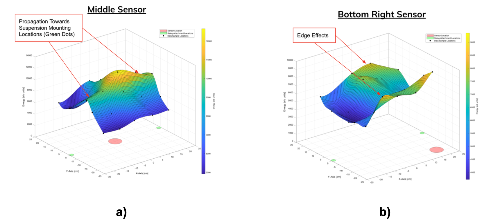
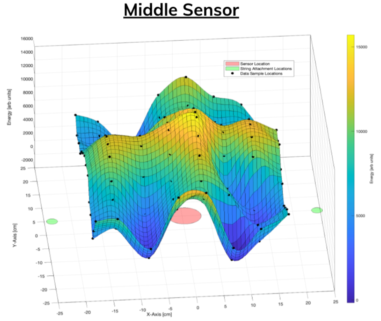
Figure 7. a) 3D cubic fit graph highlights propagation towards mounting locations b) Bottom right sensor showing edge effects

A 3D cubic fit was then used to connect all of the sample locations for each of the five sensors. The figure for the center sensor and the bottom right sensor (as an example for all 4 outside sensors) are seen in Fig. 7. It was clear that there was not a direct correlation between drop distance from the sensor and the magnitude sum. Furthermore, trends of large propagations towards the suspension mourning locations were seen along with major edge effects. Trilateration of the location of the drop would be nearly impossible given the no uniform distribution, 38% error in the sensors, and the low resolution of drops. However, the team decided that it would be very impactful if the board was broken into 9 zones (Fig. 8a) and which zone the ball landed in could be calculated. To do this, the mean and standard deviation of the portion of the 3D fit was calculated for each zone. When a sample drop was fed into the algorithm its magnitude sum would be checked to see if it was within plus or minus two standard deviations of the mean of each zone. If it was, then that zone would get an upvote. This process would then be done for all nine zones for all five sensors. Whichever zone had the most upvotes would be the zone that the team predicted the ball fell in. The heat maps for each sensor can be seen in Fig. 8b. 250 samples were passed through the algorithm and it predicted the correct location with an accuracy of 22%.

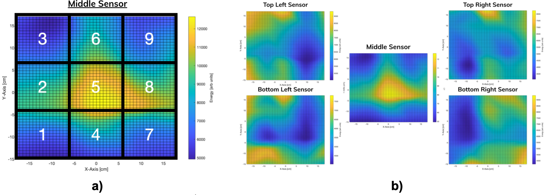
Figure 8. a) Zone numbering for 1st algorithm b) Magnitude “Heat maps” for each sensor

The team knew that there was a lot of error in the sensor measurements from previous tests, so sets of 10 drops at different locations were averaged and then fed into the algorithm. The algorithm predicted the correct location with these samples with an accuracy of 24%. While this was not what the team desired, it was roughly twice the accuracy of randomly guessing (11%). It seemed like the algorithm struggled with squares 2, 4, 6, and 8 (Fig. 8a) because there was not a sensor in those squares and the averaging and large standard deviations cause it to always guess square two because it iterated through two first. The team decided it would be worth taking a much larger, more dense data set to calibrate the board.

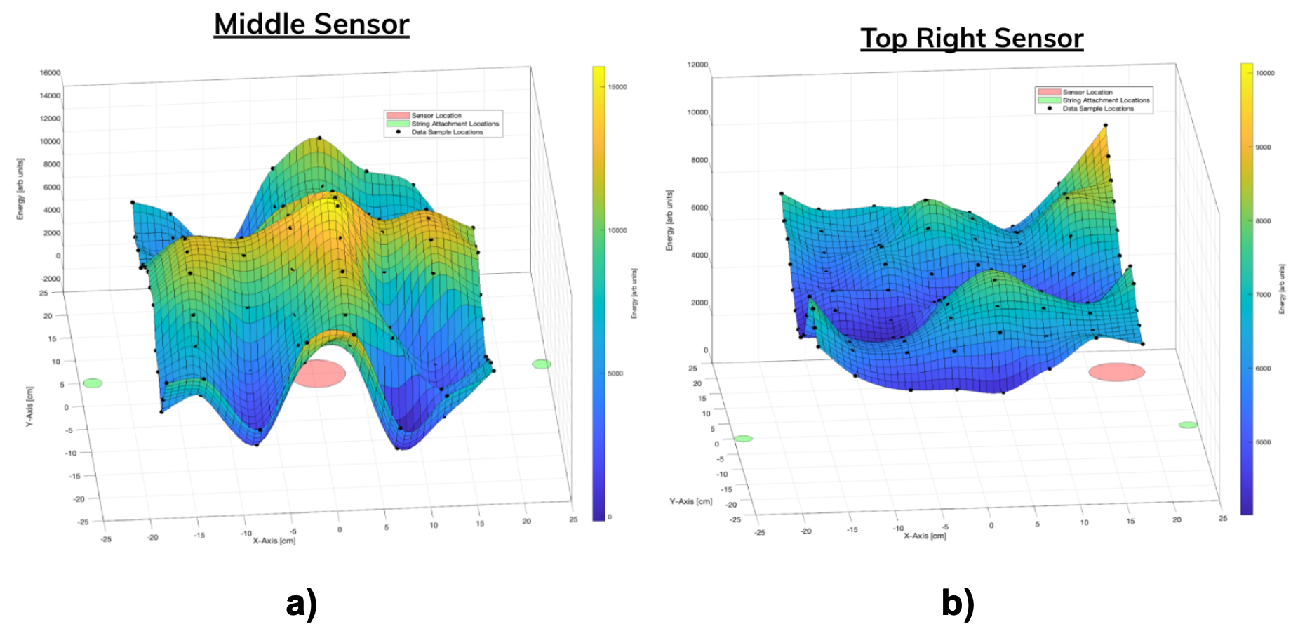
Figure 9. a) Final test 3D cubic fit graph propagation towards mounting locations exaggerated b) Bottom right sensor showing edge effects exaggerated

This time, the same error eliminating strategies were implemented but instead of 25 locations, the team dropped 10 times at 112 locations. The averages of each location were then mapped and the cubic fit for each sensor was calculated. The center sensor and bottom left sensor fits can be seen in Fig. 9. More drop locations seemed to exaggerate all of the trends seen from the “last ditch” test. Using the same algorithm the accuracy for average samples was even worse at 10.7% which was below even guessing standards (11%). It was clear that a new method for zone prediction was needed. A new algorithm was developed. For this algorithm, the board was divided into 9 zones and also 81 squares (Fig. 10b). For each square the sample magnitude sum would be compared to see if it was within 2 standard deviations of the mean of the square for every square and every sensor. Then whichever zone has the most squares with “hits” would be predicted to be the zone that the ball fell in. The accuracy of this algorithm was 49% for individual samples and 79% for 10 drops in the same location averaged. This was very exciting and demonstrated that it would be possible to use very inexpensive sensors to predict localized impacts within a ten by ten cm square with relatively high accuracy assuming a calibration was done.

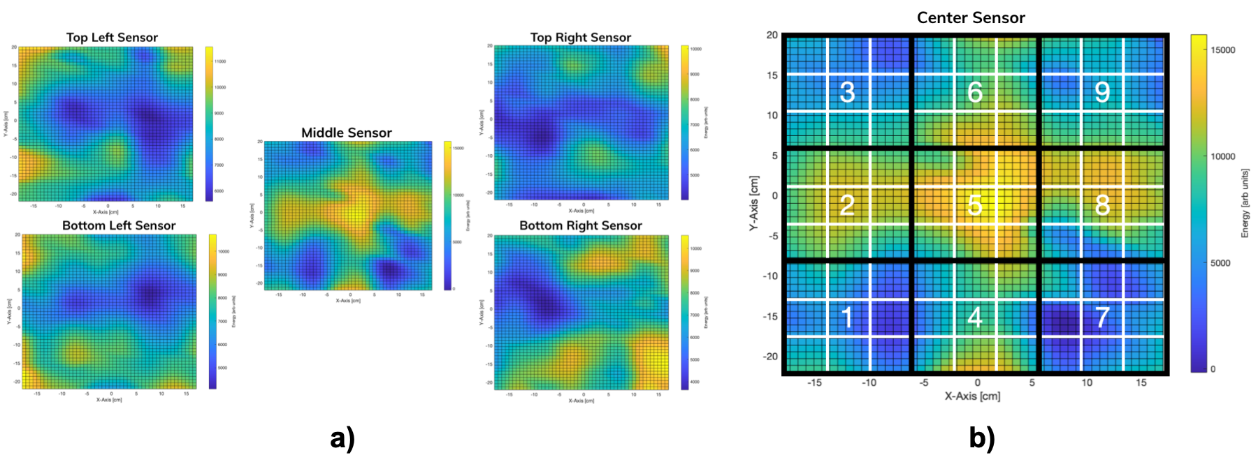
Figure 10. a) Magnitude sum “Heat maps” for each sensor b) Zone numbering and breakup for the 2nd algorithm

Discussion

The final effort to find location utilized many learnings from previous tests (notably a Riemann sum approach and filtered data to include only the first bounce) and results showed a significantly stronger correlation and algorithmic ability to determine drop location.

The algorithm was able to accurately predict the correct grid 50% of the time, but there is much room for improvement. Variation in the recorded magnitudes and true drop locations lead to less accurate predictions, as the calculated means and standard deviations for a grid are shifted from their true values due to the variations. Looking at the system then, our team determined a number of different factors that could have contributed to the poor correlation, such as inconsistencies related to ball release. From the initial uncertainty calculations, systematic error drove the total uncertainty more than random error did. Factors that notably contributed to systematic error include: material non-uniformity, relative position of sensors to drop locations, sensor attachment method to board, and piezoelectric sensor consistency. For random error, the factors observed were the true drop location and board orientation. Practically, all materials have some degree of non-uniformity throughout a given volume. That being said, using materials with higher homogeneity, such as aluminum rather than plywood, can help decrease variations in the vibrational energy that the piezoelectric sensors.

In order to decrease the systematic error created by the relative position of the sensors, a gluing fixture should be used to tightly control the position of the sensor. During the project, the sensor was hand placed with glue onto a measured position on the board. This, however, is extremely imprecise, as the installer is essentially guessing where the sensor is going as there was no physical feature to constrain the sensor position. Additionally, the liquid adhesive glue provides a slick surface for the sensor to slide on the board, which is difficult to control without a precision fixture.

The liquid adhesive used on the sensors also contributed to systematic error. Without a precision dispensing device, the volume of glue used was random, as the team would try to apply 1 layer of adhesive onto the sensor before installation. When pressing the glue and sensor onto the board, the force applied to the sensor will affect how much glue stays between the sensor and the board, which would affect the stiffness of the adhesive bond between the sensor and the board. Glue drying time also created systematic error, as data taken before a glue bond is fully cured can affect the stiffness of the adhesive bond. To decrease the systematic error contribution of the adhesive, a precision robotic dispensing device should be used, as well as a fixture to precisely control the force applied to the board with the sensors. Cure time should also be monitored and kept consistent between all the sensors.

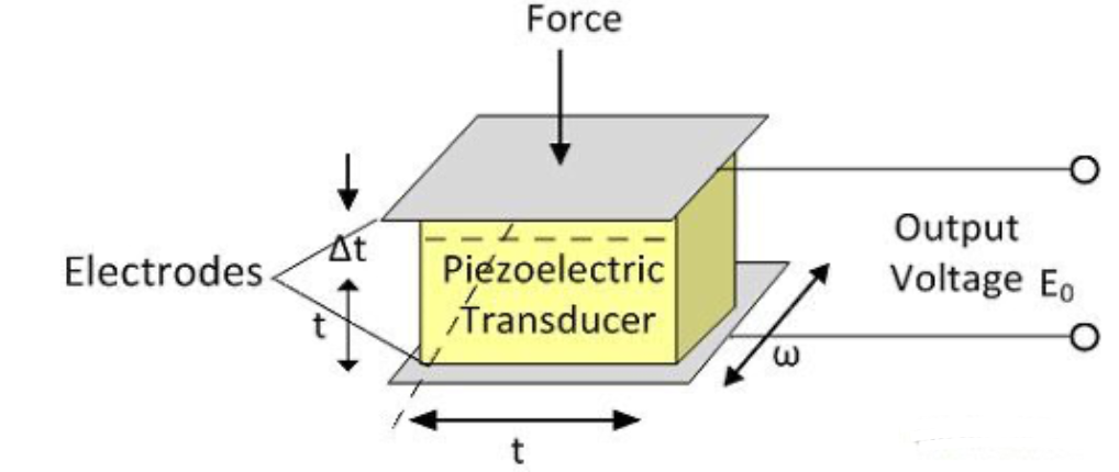
Figure 11. Breakdown of a piezoelectric sensor [3]

The components within a piezoelectric sensor also contributed to systematic error. Typically, the piezoelectric sensor is made of a crystalline material that changes voltage when mechanical deformation is experienced [2]. Variation in manufacturing and assembly processes can affect the true geometry of the piezoelectric element, which will affect the output voltage for a given deformation. In order to decrease manufacturing and assembly variation, more precise and tightly controlled processes need to be used, which will likely increase the cost per sensor.

The true impact location contributes to the random error of the system. While a custom mechanism was designed to eliminate as much variation during drop as possible (as shown in Fig. 12b), small perturbations to the fixture can affect the impact location, such as vibrations caused by the servo actuation. Tolerancing and mechanical fitment also affect the true drop location, as small forces can push internal mechanism components, causing a shift in drop position. In order to control the true impact location tightly, an improved drop fixture should be designed with stiffer structures and materials such as aluminum, while the dropper mechanism should be manufactured with highly precise processes, such as CNC Machining.

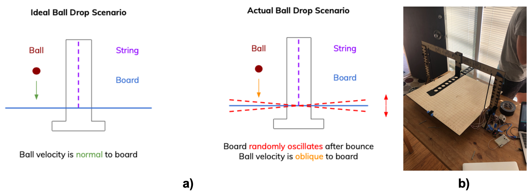
Figure 12. a) Ideal vs Actual ball drop scenarios showing uncontrolled oscillation from string dampening b) Impact board suspended by string

To eliminate the effects of damping with the board and the surface it rests on, the board was suspended off of the drop fixture. While this does eliminate damping on the sensors, it does contribute to random error, as the board is not perfectly exactly normal to the velocity of the ball drop. In fact, since it is free to rotate about its center axis, the exact angle of the board surface to the ball drop velocity vector is difficult to control. When dropping the ball onto the board, the board would randomly oscillate after the impact. Due to time constraints, ensuing ball drops were done before the board completely came to rest. Consequently, the ideally normal collision with the ball and board became randomly oblique. In order to better control the orientation of the board, allowing the board to come to rest in between ball drops would ensure a consistent orientation. That being said, the additional time in between ball drops would increase significantly, which limits the number of total ball drop data points that could be collected.

Future iterations of this project may include extension of the impact table to include different materials, multiaxial impact localization for 3D applications, higher resolution sensing, and potentially even implementing artificial intelligence towards algorithm development.

As for project applications, the team believes the findings can apply to a wide variety of industrial applications including aerospace maintenance (accurate bearing life tracking), hail damage (localized damage detection), CNC maintenance (tooling life indicator), and military/defense (impact detection).

Conclusions

Our team set out to characterize inexpensive piezoelectric vibration sensors with the ultimate goal of detecting and predicting the impact location of a dropped object onto a surface. We developed a repeatable ball drop test fixture and collected vibration data from many drops. However, the validity of the piezoelectric sensor was called into question. To further explore the data’s deviation from our initial hypotheses, we Isolated the project scope to a single dimension and used the sensor to find the height of a dropped ball. Through the completion of these tests and subsequent data analysis, we transitioned from a method of trilateration to a discretized summed magnitude-based approach that predicted the impact location on the test platform with an accuracy of 79%. This result shows that low-cost piezoelectric sensors can be utilized for impact detection applications.

References

Appendix

A) Data Acquisition Script

B) FinalAlgorithm clear clc close all %%%%%%%%%%%%%%%%%%%%%%%%%%%%%%%%%%%%%%%%%%%%%%%%%%%%%%%%%%%%%%%%%%%%%% %%%%%%%%%% % DATA IMPORT positions = readmatrix('positions2.csv'); fixy = zeros(1000,5); data1 = readmatrix('1-data.csv'); data2 = readmatrix('2-data.csv'); data3= readmatrix('3-data.csv'); data4= readmatrix('4-data2.csv'); data5= readmatrix('5-data2.csv'); data6 = readmatrix('6-data3.csv'); data7 = readmatrix('7-data2.csv'); data8 = readmatrix('8-data2.csv'); data1 = [data1(:,2:6);fixy]; data2 = [data2(:,2:6);fixy]; data3 = [data3(:,2:6);fixy]; data4 = [data4(:,2:6);fixy]; data5 = [data5(:,2:6);fixy]; data6 = [data6(:,2:6);fixy]; data7 = [data7(:,2:6);fixy]; data8 = [data8(:,2:6);fixy]; data1 = data1(1:140000,:); data2 = data2(1:140000,:); data3 = data3(1:140000,:); data4 = data4(1:140000,:); data5 = data5(1:140000,:); data6 = data6(1:140000,:); data7 = data7(1:140000,:); data8 = data8(1:140000,:); for i = 1:140000 for j = 1:5 if data1(i,j)>1023 data1(i,j)=0; end if data2(i,j)>1023 data2(i,j)=0; end if data3(i,j)>1023 data3(i,j)=0; end if data4(i,j)>1023 data4(i,j)=0; end if data5(i,j)>1023 data5(i,j)=0; end if data6(i,j)>1023 data6(i,j)=0; end if data7(i,j)>1023 data7(i,j)=0; end if data8(i,j)>1023 data8(i,j)=0; end end end data = [data1;data2;data3;data4;data5;data6;data7;data8]; 15

data(isnan(data))=0; %%%%%%%%%%%%%%%%%%%%%%%%%%%%%%%%%%%%%%%%%%%%%%%%%%%%%%%%%%%%%%%%%%%%%% %%%%%%%%%% % GENERAL VARIABLES EX = 80; %PERCENTILE OF EXCLUSIONS NSTD = 2; % NUMBER OF STDS FOR SURFACE APROX SURFACETYPE = 'cubicinterp'; % 'linearinterp' OR 'cubicinterp' SAMPLES = 112; %%%%%%%%%%%%%%%%%%%%%%%%%%%%%%%%%%%%%%%%%%%%%%%%%%%%%%%%%%%%%%%%%%%%%% %%%%%%%%%% % CALCULATING "ENERGY" OF DROPS dataSum(1,:) = sum(data(1:1000,:)); for i = 1:SAMPLES10-1 dataSum(i+1,:) = sum(data(i1000:(i+1)1000,:)); end sensorM(:,1) = dataSum(:,1); sensorBR(:,1) = dataSum(:,2); sensorBL(:,1) = dataSum(:,3); sensorTL(:,1) = dataSum(:,4); sensorTR(:,1) = dataSum(:,5); %%%%%%%%%%%%%%%%%%%%%%%%%%%%%%%%%%%%%%%%%%%%%%%%%%%%%%%%%%%%%%%%%%%%%% %%%%%%%%%%%%%% % CONNECTING LOCATIONS TO MAGNITUDES for i = 0:SAMPLES-1 for j = 1:10 sensorM(i10+j,2) = positions(i+1,1); sensorM(i10+j,3) = positions(i+1,2); sensorBR(i10+j,2) = positions(i+1,1); sensorBR(i10+j,3) = positions(i+1,2); sensorBL(i10+j,2) = positions(i+1,1); sensorBL(i10+j,3) = positions(i+1,2); sensorTL(i10+j,2) = positions(i+1,1); sensorTL(i10+j,3) = positions(i+1,2); sensorTR(i10+j,2) = positions(i+1,1); sensorTR(i10+j,3) = positions(i+1,2); end end %%%%%%%%%%%%%%%%%%%%%%%%%%%%%%%%%%%%%%%%%%%%%%%%%%%%%%%%%%%%%%%%%%%%%% %%%%%%%%%%%%%%%%%%%%%%%%%%%%%%%%%%%%%%%%%%%% % AVERAGING AND STD-ING MAGNITUDES for i= 0:SAMPLES-1 [a,a1] = rmoutliers(sensorM(i10+1:i10+10,1),'percentiles',[(100-EX)/2,(100+EX)/2]); sensorM_AVE(i+1,1) = mean(a); sensorM_AVE(i+1,4) = std(a)/sensorM_AVE(i+1,1)1500; dataSumAVE(i+1,1) = mean(a); [b,b1] = rmoutliers(sensorBR(i10+1:i10+10,1),'percentiles',[(100-EX)/2,(100+EX)/2]); sensorBR_AVE(i+1,1) = mean(b); sensorBR_AVE(i+1,4) = std(b)/sensorBR_AVE(i+1,1)1500; dataSumAVE(i+1,2) = mean(b); [c,c1] = rmoutliers(sensorBL(i10+1:i10+10,1),'percentiles',[(100-EX)/2,(100+EX)/2]); sensorBL_AVE(i+1,1) = mean(c); sensorBL_AVE(i+1,4) = std(c)/sensorBL_AVE(i+1,1)1500; dataSumAVE(i+1,3) = mean(c); [d,d1] = rmoutliers(sensorTL(i10+1:i10+10,1),'percentiles',[(100-EX)/2,(100+EX)/2]); sensorTL_AVE(i+1,1) = mean(d); sensorTL_AVE(i+1,4) = std(d)/sensorTL_AVE(i+1,1)*1500; dataSumAVE(i+1,4) = mean(d); 16

[e,e1] = rmoutliers(sensorTR(i10+1:i10+10,1),'percentiles',[(100-EX)/2,(100+EX)/2]); sensorTR_AVE(i+1,1) = mean(e); sensorTR_AVE(i+1,4) = std(e)/sensorTR_AVE(i+1,1)1500; dataSumAVE(i+1,5) = mean(e); end %%%%%%%%%%%%%%%%%%%%%%%%%%%%%%%%%%%%%%%%%%%%%%%%%%%%%%%%%%%%%%%%%%%%%% %%%%%%%%%%%%%%%%%%%%%%%%%% % MAPPING AVERAGES TO POSITIONS sensorM_AVE(:,2) = positions(1:SAMPLES,1); sensorM_AVE(:,3) = positions(1:SAMPLES,2); sensorBR_AVE(:,2) = positions(1:SAMPLES,1); sensorBR_AVE(:,3) = positions(1:SAMPLES,2); sensorBL_AVE(:,2) = positions(1:SAMPLES,1); sensorBL_AVE(:,3) = positions(1:SAMPLES,2); sensorTL_AVE(:,2) = positions(1:SAMPLES,1); sensorTL_AVE(:,3) = positions(1:SAMPLES,2); sensorTR_AVE(:,2) = positions(1:SAMPLES,1); sensorTR_AVE(:,3) = positions(1:SAMPLES,2); %%%%%%%%%%%%%%%%%%%%%%%%%%%%%%%%%%%%%%%%%%%%%%%%%%%%%%%%%%%%%%%%%%%%%% %%%%%%%%%%%%%%%%%%%%%%%%%%%%%%%%%%%%%%%%%% % GRID BREAKUP PARAMETERS range = 17; squares = 9; %zones = 16; length = 2range/squares; squares = sqrt(squares); %%%%%%%%%%%%%%%%%%%%%%%%%%%%%%%%%%%%%%%%%%%%%%%%%%%%%%%%%%%%%%%%%%%%%% %%%%%%%%%%%%%%%%%%%%%%%%%%%%%%%%%%%%%%%%%% % % MIDDLE SENSOR %%%%%%%%%%%%%%% % 3D FIT PLOT counter = 1; f = fit([sensorM_AVE(:,2), sensorM_AVE(:,3)],sensorM_AVE(:,1),SURFACETYPE); for i = -17:1:17 for j = -17:1:17 points(counter,:) = [i,j,f(i,j)]; counter = counter+1; end end F = scatteredInterpolant(points(:,1), points(:,2),points(:,3)); F.Method = 'natural'; [xq,yq] = meshgrid(-25:0.1:25); vq1 = F(xq,yq); vq1(vq1<2000)=2000; vq1(vq1>16000)=16000; %scatter3(sensorM_AVE(:,2),sensorM_AVE(:,3),sensorM_AVE(:,1),'r','filled'); hold on mesh(xq,yq,vq1); hold on p3 = scatter3 (sensorM_AVE(:,2), sensorM_AVE(:,3), sensorM_AVE(:,1),'filled','k'); p = nsidedpoly(1000, 'Center', [0 0], 'Radius', 3); p1 = plot(p, 'FaceColor', 'r'); p = nsidedpoly(1000, 'Center', [24 0], 'Radius', 1); p2 = plot(p, 'FaceColor', 'g'); p = nsidedpoly(1000, 'Center', [-24 0], 'Radius', 1); p2 = plot(p, 'FaceColor', 'g'); axis([-25,25,-25,25]); c = colorbar; % % % % % % % % % % 17

% c.Label.String = 'Energy [arb units]'; % xlabel('X-Axis [cm]') % ylabel('Y-Axis [cm]') % zlabel('Energy [arb units]') % %title('Middle Sensor','FontSize',20 ); % ax = gca; % ax.TitleHorizontalAlignment = 'left'; % legend([p1 p2 p3],{'Sensor Location','String Attachment Locations','Data Sample Locations'} ); %%%%%%%%%%%%%%% % GRABBING AVERAGES AT POINTS ON GRID count = 1; for i = 0:2range-1 for j = 0:2range-1 valuesM(i+1,j+1) = f(-range+i,-range+j); end end for i = 0:squares-1 for j = 0:squares-1 quadM(1,count) = mean((valuesM(1+lengthi:length(i+1),1+lengthj:length(j+1))),'all');%this isn't fully right quadM(2,count) = std(valuesM(1+lengthi:length(i+1),1+lengthj:length(j+1)),0,'all'); centerX = -range-length/2+(i+1)length; centerY = -range-length/2+(j+1)length; %scatter3(centerX,centerY,quadM(1,count),quadM(2,count)/5,'r','filled'); count = count + 1; end end %%%%%%%%%%%%%%% % CHECKING LOCATIONS for j = 1:size(sensorM,1) sample = sensorM(j,:); for i = 1:squares^2 locationM(j,i) = ( (quadM(1,i)-NSTDquadM(2,i)< sample(1)) && (sample(1)<quadM(1,i)+NSTDquadM(2,i))); end end % %%%%%%%%%%%%%%%%%%%%%%%%%%%%%%%%%%%%%%%%%%%%%%%%%%%%%%%%%%%%%%%%%%%%%% %%%%%%%%%%%%%%%%%%%%%%%%%%%%%%%%%%%%%%%%%% % BOTTOM RIGHT SENSOR %%%%%%%%%%%%%%% % 3D FIT PLOT figure counter = 1; g = fit([sensorBR_AVE(:,2), sensorBR_AVE(:,3)],sensorBR_AVE(:,1),SURFACETYPE); for i = -17:1:17 for j = -17:1:17 points(counter,:) = [i,j,g(i,j)]; counter = counter+1; end end G = scatteredInterpolant(points(:,1), points(:,2),points(:,3)); G.Method = 'natural'; [xq,yq] = meshgrid(-25:0.1:25); vq1 = G(xq,yq); vq1(vq1<2000)=2000; vq1(vq1>13000)=13000; %scatter3(sensorBR_AVE(:,2),sensorBR_AVE(:,3),sensorBR_AVE(:,1),'r','filled'); hold on mesh(xq,yq,vq1); hold on p = nsidedpoly(1000, 'Center', [18 -18], 'Radius', 2); plot(p, 'FaceColor', 'r'); 18

axis([-25,25,-25,25]); colorbar; %%%%%%%%%%%%%%% % GRABBING AVERAGES AT POINTS ON GRID count = 1; for i = 0:2range-1 for j = 0:2range-1 valuesBR(i+1,j+1) = g(-range+i,-range+j); end end for i = 0:squares-1 for j = 0:squares-1 quadBR(1,count) = mean((valuesBR(1+lengthi:length(i+1),1+lengthj:length(j+1))),'all');%this isn't fully right quadBR(2,count) = std(valuesBR(1+lengthi:length(i+1),1+lengthj:length(j+1)),0,'all'); centerX = -range-length/2+(i+1)length; centerY = -range-length/2+(j+1)length; %scatter3(centerX,centerY,quadM(1,count),quadM(2,count)/5,'r','filled'); count = count + 1; end end %%%%%%%%%%%%%%% % CHECKING LOCATIONS for j = 1:size(sensorBR,1) sample = sensorBR(j,:); for i = 1:squares^2 locationBR(j,i) = ( (quadBR(1,i)-NSTDquadBR(2,i)< sample(1)) && (sample(1)<quadBR(1,i)+NSTDquadBR(2,i))); end end %%%%%%%%%%%%%%%%%%%%%%%%%%%%%%%%%%%%%%%%%%%%%%%%%%%%%%%%%%%%%%%%%%%%%% %%%%%%%%%%%%%%%%%%%%%%%%%%%%%%%%%%%%%%%%%% % BOTTOM LEFT SENSOR %%%%%%%%%%%%%%% % 3D FIT PLOT figure counter = 1; h = fit([sensorBL_AVE(:,2), sensorBL_AVE(:,3)],sensorBL_AVE(:,1),SURFACETYPE); for i = -17:1:17 for j = -17:1:17 points(counter,:) = [i,j,h(i,j)]; counter = counter+1; end end H = scatteredInterpolant(points(:,1), points(:,2),points(:,3)); H.Method = 'natural'; [xq,yq] = meshgrid(-25:0.1:25); vq1 = H(xq,yq); vq1(vq1<2000)=2000; vq1(vq1>15000)=15000; %scatter3(sensorBL_AVE(:,2),sensorBL_AVE(:,3),sensorBL_AVE(:,1),'r','filled'); hold on mesh(xq,yq,vq1); hold on p = nsidedpoly(1000, 'Center', [-18 -18], 'Radius', 2); plot(p, 'FaceColor', 'r'); axis([-25,25,-25,25]); colorbar; %%%%%%%%%%%%%%% % GRABBING AVERAGES AT POINTS ON GRID count = 1; for i = 0:2*range-1 19

for j = 0:2range-1 valuesBL(i+1,j+1) = h(-range+i,-range+j); end end for i = 0:squares-1 for j = 0:squares-1 quadBL(1,count) = mean((valuesBL(1+lengthi:length*(i+1),1+lengthj:length(j+1))),'all');%this isn't fully right quadBL(2,count) = std(valuesBL(1+lengthi:length(i+1),1+lengthj:length(j+1)),0,'all'); centerX = -range-length/2+(i+1)length; centerY = -range-length/2+(j+1)length; %scatter3(centerX,centerY,quadM(1,count),quadM(2,count)/5,'r','filled'); count = count + 1; end end %%%%%%%%%%%%%%% % CHECKING LOCATIONS for j = 1:size(sensorBL,1) sample = sensorBL(j,:); for i = 1:squares^2 locationBL(j,i) = ( (quadBL(1,i)-NSTDquadBL(2,i)< sample(1)) && (sample(1)<quadBL(1,i)+NSTDquadBL(2,i))); end end %%%%%%%%%%%%%%%%%%%%%%%%%%%%%%%%%%%%%%%%%%%%%%%%%%%%%%%%%%%%%%%%%%%%%% %%%%%%%%%%%%%%%%%%%%%%%%%%%%%%%%%%%%%%%%%% % TOP LEFT SENSOR %%%%%%%%%%%%%%% % 3D FIT PLOT figure counter = 1; r = fit([sensorTL_AVE(:,2), sensorTL_AVE(:,3)],sensorTL_AVE(:,1),SURFACETYPE); for i = -17:1:17 for j = -17:1:17 points(counter,:) = [i,j,r(i,j)]; counter = counter+1; end end R = scatteredInterpolant(points(:,1), points(:,2),points(:,3)); R.Method = 'natural'; [xq,yq] = meshgrid(-25:0.1:25); vq1 = R(xq,yq); vq1(vq1<2000)=2000; vq1(vq1>13000)=13000; scatter3(sensorTL_AVE(:,2),sensorTL_AVE(:,3),sensorTL_AVE(:,1),'r','filled'); hold on mesh(xq,yq,vq1); hold on p = nsidedpoly(1000, 'Center', [-18 18], 'Radius', 2); plot(p, 'FaceColor', 'r'); axis([-25,25,-25,25]); colorbar; %%%%%%%%%%%%%%% % GRABBING AVERAGES AT POINTS ON GRID count = 1; for i = 0:2range-1 for j = 0:2range-1 valuesTL(i+1,j+1) = r(-range+i,-range+j); end end for i = 0:squares-1 for j = 0:squares-1 20

quadTL(1,count) = mean((valuesTL(1+lengthi:length(i+1),1+lengthj:length(j+1))),'all');%this isn't fully right quadTL(2,count) = std(valuesTL(1+lengthi:length(i+1),1+lengthj:length(j+1)),0,'all'); centerX = -range-length/2+(i+1)length; centerY = -range-length/2+(j+1)length; %scatter3(centerX,centerY,quadM(1,count),quadM(2,count)/5,'r','filled'); count = count + 1; end end %%%%%%%%%%%%%%% % CHECKING LOCATIONS for j = 1:size(sensorTL,1) sample = sensorTL(j,:); for i = 1:squares^2 locationTL(j,i) = ( (quadTL(1,i)-NSTDquadTL(2,i)< sample(1)) && (sample(1)<quadTL(1,i)+NSTDquadTL(2,i))); end end %%%%%%%%%%%%%%%%%%%%%%%%%%%%%%%%%%%%%%%%%%%%%%%%%%%%%%%%%%%%%%%%%%%%%% %%%%%%%%%%%%%%%%%%%%%%%%%%%%%%%%%%%%%%%%%% % TOP RIGHT SENSOR %%%%%%%%%%%%%%% % 3D FIT PLOT figure counter = 1; q = fit([sensorTR_AVE(:,2), sensorTR_AVE(:,3)],sensorTR_AVE(:,1),SURFACETYPE); for i = -17:1:17 for j = -17:1:17 points(counter,:) = [i,j,q(i,j)]; counter = counter+1; end end Q = scatteredInterpolant(points(:,1), points(:,2),points(:,3)); Q.Method = 'natural'; [xq,yq] = meshgrid(-25:0.1:25); vq1 = Q(xq,yq); vq1(vq1<2000)=2000; vq1(vq1>13000)=13000; %scatter3(sensorTR_AVE(:,2),sensorTR_AVE(:,3),sensorTR_AVE(:,1),'r','filled'); mesh(xq,yq,vq1); hold on p3 = scatter3 (sensorTR_AVE(:,2), sensorTR_AVE(:,3), sensorTR_AVE(:,1),'filled','k'); p = nsidedpoly(1000, 'Center', [18 18], 'Radius', 3); p1 = plot(p, 'FaceColor', 'r'); p = nsidedpoly(1000, 'Center', [24 0], 'Radius', 1); p2 = plot(p, 'FaceColor', 'g'); p = nsidedpoly(1000, 'Center', [-24 0], 'Radius', 1); p2 = plot(p, 'FaceColor', 'g'); % axis([-25,25,-25,25]); c = colorbar; c.Label.String = 'Energy [arb units]'; xlabel('X-Axis [cm]') ylabel('Y-Axis [cm]') zlabel('Energy [arb units]') %title('Middle Sensor','FontSize',20 ); ax = gca; ax.TitleHorizontalAlignment = 'left'; legend([p1 p2 p3],{'Sensor Location','String Attachment Locations','Data Sample Locations'} ); %%%%%%%%%%%%%%% % GRABBING AVERAGES AT POINTS ON GRID count = 1; for i = 0:2range-1 for j = 0:2range-1 valuesTR(i+1,j+1) = q(-range+i,-range+j); 21

end end for i = 0:squares-1 for j = 0:squares-1 quadTR(1,count) = mean((valuesTR(1+lengthi:length(i+1),1+lengthj:length(j+1))),'all');%this isn't fully right quadTR(2,count) = std(valuesTR(1+lengthi:length(i+1),1+lengthj:length(j+1)),0,'all'); centerX = -range-length/2+(i+1)length; centerY = -range-length/2+(j+1)length; %scatter3(centerX,centerY,quadM(1,count),quadM(2,count)/5,'r','filled'); count = count + 1; end end %%%%%%%%%%%%%%% % CHECKING LOCATIONS for j = 1:size(sensorTR,1) sample = sensorTR(j,:); for i = 1:squares^2 locationTR(j,i) = ( (quadTR(1,i)-NSTDquadTR(2,i)< sample(1)) && (sample(1)<quadTR(1,i)+NSTDquadTR(2,i))); end end %%%%%%%%%%%%%%%%%%%%%%%%%%%%%%%%%%%%%%%%%%%%%%%%%%%%%%%%%%%%%%%%%%%%%% %%%%%%%%%%%%%%%%%%%%%%%%%%%%%%%%%%%%%%%%%% % FINAL ZONE CALC location = locationM+locationBR + locationBL + locationTL + locationTR; for i = 1:250 [quad(2,i),quad(1,i)] = max(location(i,:)); end quad = quad'; %%%%%%%%%%%%%%% % SQUARE GAMES for z = 1:size(sensorM) testSample = dataSum(z,:); range = 50; bigSquares = 9; littleSquares = 81; sqLength = 46/9; sqSTD = 1000; for i = 1:sqrt(littleSquares) for j = 1:sqrt(littleSquares) Msqmean (j,i) = F(-range/2+.5sqLength + sqLength(i-1),range/2-.5sqLength - sqLength(j-1)); MnumSquare(j,i) = ((testSample(1,1) > Msqmean(j,i)-sqSTD)&&(testSample(1,1) < Msqmean(j,i)+sqSTD)); BRsqmean (j,i) = G(-range/2+.5sqLength + sqLength(i-1),range/2-.5sqLength - sqLength(j-1)); BRnumSquare(j,i) = ((testSample(1,2) > BRsqmean(j,i)-sqSTD)&&(testSample(1,2) < BRsqmean(j,i)+sqSTD)); BLsqmean (j,i) = H(-range/2+.5sqLength + sqLength(i-1),range/2-.5sqLength - sqLength(j-1)); BLnumSquare(j,i) = ((testSample(1,3) > BLsqmean(j,i)-sqSTD)&&(testSample(1,3) < BLsqmean(j,i)+sqSTD)); TLsqmean (j,i) = R(-range/2+.5sqLength + sqLength(i-1),range/2-.5sqLength - sqLength(j-1)); TLnumSquare(j,i) = ((testSample(1,4) > (TLsqmean(j,i)-sqSTD))&&(testSample(1,4) < (TLsqmean(j,i)+sqSTD))); TRsqmean (j,i) = Q(-range/2+.5sqLength + sqLength(i-1),range/2-.5sqLength - sqLength(j-1)); TRnumSquare(j,i) = ((testSample(1,5) > TRsqmean(j,i)-sqSTD)&&(testSample(1,5) < TRsqmean(j,i)+sqSTD)); sensorM(:,1) = dataSum(:,1); end end sqMean = MnumSquare + BRnumSquare + BLnumSquare + TRnumSquare + TLnumSquare ; sqLocation = zeros(sqrt(bigSquares),sqrt(bigSquares)); for i = 0:sqrt(bigSquares)-1 for j = 0:sqrt(bigSquares)-1 for l = 1:sqrt(bigSquares) for s = 1:sqrt(bigSquares) sqLocation(j+1,i+1) = sqLocation(j+1,i+1) + sqMean(sqrt(bigSquares)*j+s,sqrt(bigSquares)*i+l); end end end 22

end sqLocation = [sqLocation(3,1),sqLocation(2,1),sqLocation(1,1),sqLocation(3,2),sqLocation(2,2),sqLocation(1,2),sqLocation(3,3),sqLocation(2,3),s qLocation(1,3)]; [sqLOCS(2,z),sqLOCS(1,z)] = max(sqLocation(:)); end sqLOCS = sqLOCS';

When writing your article, use Mathpix Markdown (which has extended LaTeX features) or regular Markdown.

References

- Korotčenkov Gennadij Sergeevič, and Korotčenkov Gennadij Sergeevič. Handbook of Gas Sensor Materials: Properties, Advantages and Shortcomings for Applications, Springer, New York, 2013.
- “Piezo Terminology & Glossary.” PIEZO.COM, https://piezo.com/pages/piezo-terminology-glossary#d.
- 11, YOGESHWARAN P April, et al. “What Is Piezo-Electric Transducer? - Definition, Piezo-Electric Effect, Theory, Properties & Uses.” Circuit Globe, 18 Aug. 2017, https://circuitglobe.com/piezo-electric-transducer.html.
- “Logging Arduino Serial Output to CSV/Excel (Windows/Mac/Linux).” Logging Arduino Serial Output to CSV/Excel (Windows/Mac/Linux) - Circuit Journal, https://circuitjournal.com/arduino-serial-to-spreadsheet.