This is the lecture notes from Chandra Chekuri's CS583 course on Approximation Algorithms. Chapter 13: Survivable Network Design Problem.
You can read Chapter 14: Introduction to Cut and Partitioning Problems, here. Chapter 12: Primal Dual for Constrained Forest Problems, here.
Chapter 13
In this chapter we consider the Survivable Network Design Problem problem. The input is an undirected graph G=(V,E)G=(V, E) with edge-weights c:E rarrR_(+)c: E \rightarrow \mathbb{R}_{+} and integer requirements r(uv)r(u v) for each pair of vertices uvu v. We wrote uvu v instead of (u,v)(u, v) to indicate that the requirement function is for unordered pairs (alternatively, r(u,v)=r(v,u)r(u, v)=r(v, u) for all u,vu, v). The goal is to find a min-cost subgraph H=(V,F)H=(V, F) of GG such that each the connectivity betweeen uu and vv in HH is at least r(uv)r(u v). We obtain two versions of the problem: EC-SNDP if the connectivity requirement is edge-connectivity and VC-SNDP for vertex connectivity. It turns out that EC-SNDP is much more tractable than VC-SNDP and we will focus on EC-SNDP.
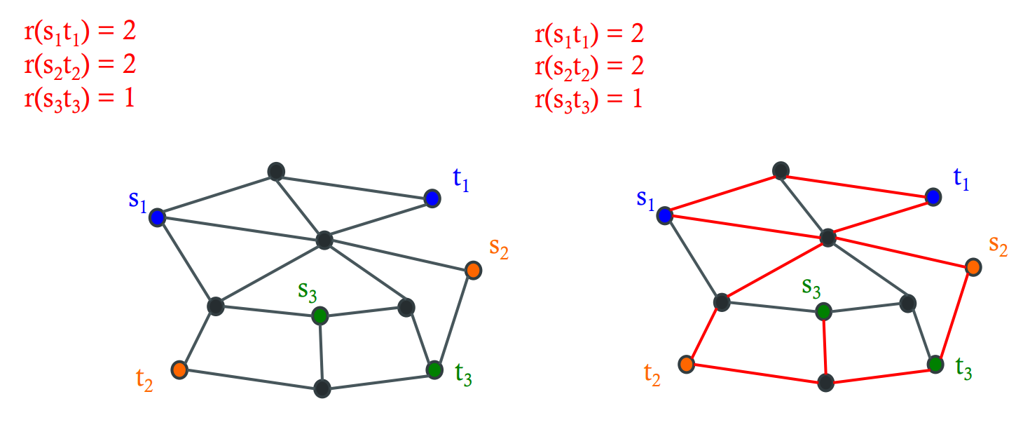
Figure 13.1: Example of EC-SNDP. Requirement only for three pairs. A feasible solution shown in the second figure as red edges. In this example the paths for each pair are also vertex disjoint even though the requirement is only for edge-disjointness.
For EC-SNDP there is a seminal work of Jain based on iterated rounding that yields a 2-approximation as a special case of a more general problem. Prior to his work there was an augmentation based approach that yields 2k2 k and 2H_(k)2 H_{k} approximations where k=max_(uv)r(uv)k=\max _{u v} r(u v) is the maximum connectivity requirement. Despite being superceded by Jain's result in terms of the ratio, the augmentation approach is important for various reasons and we will discuss both.
We first consider the LP relaxation for the EC-SNDP. We do this by setting up the requirement function f:2^(V)rarrZf: 2^{V} \rightarrow \mathbb{Z} where we let f(S)=max_(u in S,v in V-S)r(uv)f(S)=\max _{u \in S, v \in V-S} r(u v). The goal is to find a min-cost subgraph HH of GG such that delta_(H)(S) >= f(S)\delta_{H}(S) \geq f(S).
Claim 13.0.1.The requirement functionffthat captures EC-SNDP is proper and hence skew-supermodular.
Proof. It is easy to see ff is symmetric. Consider disjoint sets A,BA, B. Suppose f(A uu B)=kf(A \cup B)=k which means that there is some s in A uu Bs \in A \cup B and t in V-(A uu B)t \in V-(A \cup B) such that r(st)=kr(s t)=k. If s in As \in A then f(A) >= kf(A) \geq k and if s in Bs \in B then f(B) >= kf(B) \geq k. Therefore max{f(A),f(B)} >= k=f(A uu B)\max \{f(A), f(B)\} \geq k=f(A \cup B) since s in As \in A or s in Bs \in B.
13.1 Augmentation approach
The augmentation approach for EC-SNDP is based on iteratively increasing the connectivity of pairs from 11 to kk where k=max_(uv)r(uv)k=\max _{u v} r(u v). In fact this works for any proper function f:2^(V)rarrZf: 2^{V} \rightarrow \mathbb{Z} and we will work in this generality rather than focus only on EC-SNDP.
Claim 13.1.1.Letffbe a proper function and letppbe an integer. Then the truncated functiong_(p):2^(V)rarrZg_{p}: 2^{V} \rightarrow \mathbb{Z}defined asg_(p)(S)=min{p,f_(p)(S)}g_{p}(S)=\min \left\{p, f_{p}(S)\right\}is proper.
Proof. Exercise.
Lemma 13.1.LetG=(V,E)G=(V, E)be graph and letf:2^(V)rarrZf: 2^{V} \rightarrow \mathbb{Z}be a proper function and letp >= 0p \geq 0be a non-negative integer. LetX sube EX \subseteq Ebe a set of edges such that|delta_(X)(S)| >= g_(p)(S)\left|\delta_{X}(S)\right| \geq g_{p}(S)Consider the functionh_(p+1):2^(V)rarr{0,1}h_{p+1}: 2^{V} \rightarrow\{0,1\}whereh_(p+1)(S)=1h_{p+1}(S)=1ifff(S) >= p+1f(S) \geq p+1and|delta_(X)(S)|=p\left|\delta_{X}(S)\right|=p. Thenh_(p+1)h_{p+1}is uncrossable and symmetric.
Proof. Consider the function g_(p+1)g_{p+1} which is proper and hence also skew-supermodular. For notational convenience we use hh for h_(p+1)h_{p+1}. Suppose h(A)=h(B)=1h(A)=h(B)=1. This implies g_(p+1)(A) >= p+1g_{p+1}(A) \geq p+1 and g_(p+1)(B) >= p+1g_{p+1}(B) \geq p+1 and |delta_(X)(A)|=delta_(X)(B)=p\left|\delta_{X}(A)\right|=\delta_{X}(B)=p. g_(p+1)g_{p+1} is skewsupermodular. First case is when g_(p+1)(A)+g_(p+1)(B) <= g_(p+1)(A uu B)+g_(p+1)(A nn B)g_{p+1}(A)+g_{p+1}(B) \leq g_{p+1}(A \cup B)+g_{p+1}(A \cap B). This implies that g_(p+1)(A uu B)=g_(p+1)(B)=p+1g_{p+1}(A \cup B)=g_{p+1}(B)=p+1. By submodularity of |delta_(X)|\left|\delta_{X}\right| we have |delta_(X)(A)|+|delta_(X)(B)| >= |delta_(X)(A nn B)|+|delta_(X)(A uu B)|\left|\delta_{X}(A)\right|+\left|\delta_{X}(B)\right| \geq\left|\delta_{X}(A \cap B)\right|+\left|\delta_{X}(A \cup B)\right| and by feasibility of XX for g_(p)g_{p} we have |delta_(X)(A nn B)|=|delta_(X)(A nn B)|=p\left|\delta_{X}(A \cap B)\right|=\left|\delta_{X}(A \cap B)\right|=p. This implies that h(A nn B)=h(A uu B)=1h(A \cap B)=h(A \cup B)=1.
Similarly, if g_(p+1)(A)+g_(p+1)(B) <= g_(p+1)(A-B)+g_(p+1)(B-A)g_{p+1}(A)+g_{p+1}(B) \leq g_{p+1}(A-B)+g_{p+1}(B-A) we can argue that h(A-B)=h(B-A)=1h(A-B)=h(B-A)=1 via posi-modularity of |delta_(X)|\left|\delta_{X}\right|.
Exercise 13.1. Let G=(V,E)G=(V, E) be a graph and let f:2^(V)rarrZf: 2^{V} \rightarrow \mathbb{Z} be a proper function. Suppose FF be a feasible cover for g_(p)g_{p}. Let h_(p+1)h_{p+1} be the residulal uncrossable function that arises from g_(p)g_{p} as in the preceding lemma. Let F^(')sube E\\FF^{\prime} \subseteq E \backslash F be a feasible cover for h_(p+1)h_{p+1} in the graph G^(')=(V,E\\F)G^{\prime}=(V, E \backslash F). Then F uuF^(')F \cup F^{\prime} is a feasible cover for g_(p+1)g_{p+1}.
Lemma 13.2.Letffbe the requirement function of an instance of EC-SNDP inG=(V,E)G=(V, E)and letppbe an integer and letX sube EX \subseteq Ebe a set of edges. There is a polynomial time algorithm to find the minimal violated sets ofg_(p)g_{p}with respect toXX.
Proof. For each pair or nodes (s,t)(s, t) find a source-minimal s-ts-t mincut SS in the graph H=(V,X)H=(V, X) and a sink-minimal mincut TT via maxflow[1]. Let SS be the cut. If |delta_(X)(S)| < p\left|\delta_{X}(S)\right|<p then pp is a violated set. We compute all such minimal cuts over all pairs of vertices and take the minimal sets in this collection. We leave it as an exercise to check that the minimal violated sets of g_(p)g_{p} are the minimal sets in this collection and will be disjoint.
Corollary 13.1.Letffbe the requirement function of an instance of EC-SNDP inG=(V,E)G=(V, E)and letppbe an integer. LetXXbe set of edges such thatXXis feasible to coverg_(p)g_{p}. In the graphG^(')=(V,E\\X)G^{\prime}=(V, E \backslash X)and for anyF sube(E\\X)F \subseteq(E \backslash X)the minimal violated sets ofh_(p+1)h_{p+1}with respect toFFcan computed in polynomial time.
Proof. The minimial violated sets of h_(p+1)h_{p+1} with respect to FF are the same as the minimal violated sets of g_(p+1)g_{p+1} with respect to X uu FX \cup F.
2. k=max_(S)f(S)k=\max _{S} f(S) is the maximum requirement
3. A longleftarrow O/A \longleftarrow \emptyset
4. for (p=1(p=1 to k)k) do
quad\quad A. G^(')=(V,E\\A)G^{\prime}=(V, E \backslash A)
quad\quad B. Let g_(p)g_{p} be the function defined as g_(p)(S)=min{f(S),p}g_{p}(S)=\min \{f(S), p\}
quad\quad C. Let h_(p)h_{p} be the uncrossable function where h_(p)(S)=1h_{p}(S)=1 iff g_(p)(S) > |delta_(A)(S)|g_{p}(S)>\left|\delta_{A}(S)\right|
quad\quad D. Find A^(')sube E\\AA^{\prime} \subseteq E \backslash A that covers h_(p)h_{p} in G^(')G^{\prime}
quad\quad E. A larr A uuA^(')A \leftarrow A \cup A^{\prime}
5. Output AA
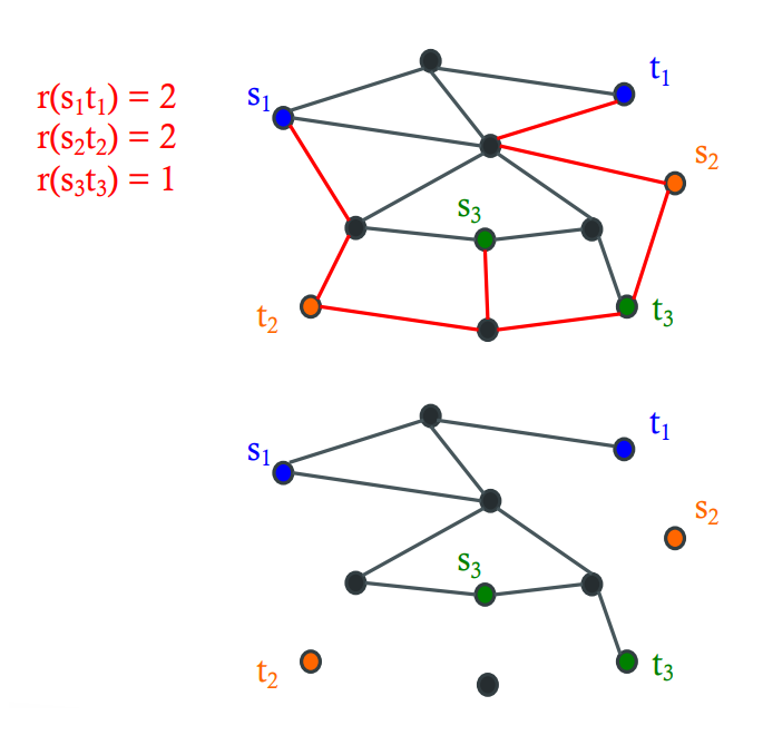
Figure 13.2: Example to illustrate the augmentation approach. Top picture shows a set of edges that connect all pairs with connectivity requirement at least 11. Second picture shows the residual graph in which one needs to solve the augmentation problem. Note that s_(2)s_{2} and t_(2)t_{2} are isolated vertices in the residual graph, however, the cuts induced by them are already satisfied by the edges chosen in the first iteration.
Theorem 13.2.The augmentation algorithm yields a2k2 k-approximation for EC-SNDP wherekkis the maximum connectivity requirement.
Proof. We sketch the proof. The algorithm has kk iterations and in each iteration it uses a black box algorithm to cover an uncrossable function. We saw a primaldual 22-approximation for this problem. We observe that if F^(**)F^{*} is an optimum solution to the given instance then in each iteration F^(**)\\AF^{*} \backslash A is a feasible solution to the covering problem in that iteration. Thus the cost paid by the algorithm in each iteration can be bound by 2c(F^(**))2 c\left(F^{*}\right) and hence the total cost is at most 2k2 k OPT. The preceding lemmas argue that the primal-dual algorithm can be implemented in polynomial time.
Remark 13.1. A different algorithm that is based on augmentation in reverse yields a 2H_(k)2 H_{k} approximation where H_(k)H_{k} is the k^(')k^{\prime}th harmonic number. We refer the reader to [2].
13.2 Iterated rounding based 2-approximation
In the section we describe the seminal result of Jain [3] who obtained a 22-approximation for EC-SNDP via iterated rounding. He proved a more general polyhedral result. Consider the problem of covering a skew-supermodular function f:2^(V)rarrZf: 2^{V} \rightarrow \mathbb{Z} by the edges of a graph G=(V,E)G=(V, E). The natural cut covering LP relaxation for the problem is given below.
{:[minsum_(e in E)c(e)x_(e)],[sum_(e in delta(S))x_(e) >= f(S)quad S sub V],[x_(e) in[0","1]quad e in E]:}\begin{aligned}
\min \sum_{e \in E} c(e) x_{e} & \\
\sum_{e \in \delta(S)} x_{e} & \geq f(S) \quad S \subset V \\
x_{e} & \in[0,1] \quad e \in E
\end{aligned}
Note that upper bound constraints x_(e) <= 1x_{e} \leq 1 are necessary in the general setting when ff is integer valued since we can only take one copy of an edge. The key structural theorem of Jain is the following.
Theorem 13.3.Letxxbe a basic feasible solution to the LP relaxation. Then there is some edgee in Ee \in Esuch thatx_(e)=0x_{e}=0orx_(e) >= 1//2x_{e} \geq 1 / 2.
With the above in place, and the observation that the residual function of a skew-supermodular function is again a skew-supermodular function, one obtains an interative rounding algorithm.
Corollary 13.4.The integrality gap of the cut LP is at most22for any skew-supermodular functionff.
Proof. We consider the iterative rounding algorithm and prove the result via induction on mm the number of edges in GG. The base case of m=0m=0 is trivial since the function has to be 00.
Let x^(**)x^{*} be an optimum basic feasible solution to the LP relaxation. We have sum_(e in E)c_(e)x_(e)^(**) <=\sum_{e \in E} c_{e} x_{e}^{*} \leq OPT. We can assume without loss of generality that ff is not trivial in the sense that f(S) >= 1f(S) \geq 1 for at least some set SS, otherwise x=0x=0 is optimal and there is nothing to prove. By Theorem 13.3, there is an edge tilde(e)in E\tilde{e} \in E such that x_( tilde(e))^(**)=0x_{\tilde{e}}^{*}=0 or x_( tilde(e))^(**) >= 1//2x_{\tilde{e}}^{*} \geq 1 / 2. Let E^(')=E\\ tilde(e)E^{\prime}=E \backslash \tilde{e} and G^(')=(V,E^('))G^{\prime}=\left(V, E^{\prime}\right). In the former case we can discard tilde(e)\tilde{e} and the current LP solution restricted to E^(')E^{\prime} is a feasible fractional solution and we obtain the desired result via induction since we have one less edge.
The more interesting case is when x_( tilde(e))^(**) >= 1//2x_{\tilde{e}}^{*} \geq 1 / 2. The algorithm includes tilde(e)\tilde{e} and recurses on G^(')G^{\prime} and the residual function g:2^(V)rarrZg: 2^{V} \rightarrow \mathbb{Z} where g(S)=f(S)-|delta_( tilde(e))(S)|g(S)=f(S)-\left|\delta_{\tilde{e}}(S)\right|. Note that gg is skew-supermodular. We observe that A^(')subeE^(')A^{\prime} \subseteq E^{\prime} is a feasible solution to cover gg in G^(')G^{\prime} iff A^(')uu{ tilde(e)}A^{\prime} \cup\{\tilde{e}\} is a feasible solution to cover ff in GG. Furthermore, we also observe that the fractional solution x^(')x^{\prime} obtained by restricting xx to E^(')E^{\prime} is a feasible fractional solution to the LP relaxation to cover gg in G^(')G^{\prime}. Thus, by induction, there is a solution A^(')subeE^(')A^{\prime} \subseteq E^{\prime} such that c(A^(')) <= 2sum_(e inE^('))c(e)x_(e)^(**)c\left(A^{\prime}\right) \leq 2 \sum_{e \in E^{\prime}} c(e) x_{e}^{*}. The algorithm outputs A=A^(')uu{ tilde(e)}A=A^{\prime} \cup\{\tilde{e}\} which is feasible to cover ff in GG. We have
We used the fact that x_( tilde(e))^(**) >= 1//2x_{\tilde{e}}^{*} \geq 1 / 2 to upper bound c( tilde(e))c(\tilde{e}) by 2c( tilde(e))x_( tilde(e))^(**)2 c(\tilde{e}) x_{\tilde{e}}^{*}.
2-approximation for EC-SNDP : We had already seen that the requirement function for EC-SNDP is skew-supermodular. To applyTheorem 13.3 and obtain a 2-approximation for EC-SNDP we need to argue that the LP relaxation can be solved efficiently. We observe that the LP relaxation at the top level can be solved efficiently via maxflow. We need to check that in the graph GG with edge capacities given by the fractional solution xx the min-cut between every pair of vertices (s,t)(s, t) is at least r(s,t)r(s, t). Note that the algorithm is iterative. As we proceed the function g=f_(A)g=f_{A} where ff is the original requirement function and the AA is the set of edges already chosen.
Exercise 13.2. Prove that there is an efficient separation oracle for each step of the iterative rounding algorithm when ff is the requirement function for a given EC-SNDP instance.
We now prove Theorem 13.3. The proof consists of two steps. The first step is a characterization of basic feasible solutions via laminar tight sets. The second step is a counting argument.
13.2.1 Basic feasible solutions and laminar family of tight sets
Let xx be a basic feasible solution to the LP relaxation. We are done if there is any edge ee such that x_(e)=0x_{e}=0 or x_(e)=1x_{e}=1. Hence the interesting case is when xx is fully fractional, that is, x_(e)in(0,1)x_{e} \in(0,1) for every e in Ee \in E.
Definition 13.5.A setS sube VS \subseteq Vis tight with respect toxxifx(delta(S))=f(S)x(\delta(S))=f(S).
The LP relaxation is of the form Ax >= b,x in[0,1]^(m)A x \geq b, x \in[0,1]^{m}. We number the edges as e_(1),e_(2),dots,e_(m)e_{1}, e_{2}, \ldots, e_{m} arbitarily. Note that each row of AA corresponds to a set SS and the non-zero entries in the row corresponding to SS are precisely for edges in delta(S)\delta(S). For notational convenience we use chi_(S)\chi_{S} to denote the mm-dimensional row vector where chi_(S)(i)=0\chi_{S}(i)=0 if e_(i)!in delta(S)e_{i} \notin \delta(S) and chi_(S)(i)=1\chi_{S}(i)=1 if e in delta(S)e \in \delta(S). By the rank lemma, if xx is a basic feasible solution that is fully fractional, then there are mm tight sets S_(1),S_(2),dots,S_(m)S_{1}, S_{2}, \ldots, S_{m} such that the vectors chi_(S_(1)),chi_(S_(2)),dots,chi_(S_(m))\chi_{S_{1}}, \chi_{S_{2}}, \ldots, \chi_{S_{m}} are linearly independent in R^(m)\mathbb{R}^{m}. In other words xx is the unique solution to the system chi_(S_(i))^(T)x=f(S_(i)),1 <= i <= m\chi_{S_{i}}^{T} x=f\left(S_{i}\right), 1 \leq i \leq m. Note that for a given basic feasible solution xx there can be many such bases. A key technical lemma is that one choose a nice one.
Lemma 13.3.Letxxbe a basic feasible solution to the cut covering LP relaxation of a skew-supermodular functionffwherex_(e)in(0,1)x_{e} \in(0,1)for allee. Then there is a laminar familyL\mathcal{L}of tight setsS_(1),S_(2),dots,S_(m)S_{1}, S_{2}, \ldots, S_{m}such thatxxis the unique solution to the systemchi_(S_(i))^(T)x=f(S_(i))\chi_{S_{i}}^{T} x=f\left(S_{i}\right).
Figure 13.3: Laminar family of tight sets.
We need an auxiliary uncrossing lemma.
Lemma 13.4.SupposeAAandBBare two tight sets with respect toxxsuch thatA,BA, Bcross. Then one of the following holds:
•A nn B,A uu BA \cap B, A \cup Bare tight andchi_(A)+chi_(B)=chi_(A uu B)+chi_(A nn B)\chi_{A}+\chi_{B}=\chi_{A \cup B}+\chi_{A \cap B}.
Proof. Since ff is skew-supermodular f(A)+f(B) <= f(A nn B)+f(A uu B)f(A)+f(B) \leq f(A \cap B)+f(A \cup B) or f(A)+f(B) <= f(A-B)+f(B-A)f(A)+f(B) \leq f(A-B)+f(B-A). We will consider the first case.
A,BA, B are tight, hence x(delta(A))=f(A)x(\delta(A))=f(A) and x(delta(B))=f(B)x(\delta(B))=f(B). Moreover the function h(S)=x(delta(S))h(S)=x(\delta(S)) is submodular (recall that the cut capacity function in an undirected graph is symmetric submodular). Thus x(delta(A))+x(delta(B)) >=x(\delta(A))+x(\delta(B)) \geqx(delta(A uu B))+x(delta(A nn B))x(\delta(A \cup B))+x(\delta(A \cap B)). We also have by feasibility of xx that x(delta(A uu B)) >= f(A uu B)x(\delta(A \cup B)) \geq f(A \cup B) nad x(delta(A nn B)) >= f(A nn B)x(\delta(A \cap B)) \geq f(A \cap B). Putting together we have
x(delta(A))+x(delta(B))=f(A)+f(B) <= f(A nn B)+f(A uu B) <= x(delta(A uu B))+x(delta(A nn B)) <= x(delta(A))+x(delta(B)).x(\delta(A))+x(\delta(B))=f(A)+f(B) \leq f(A \cap B)+f(A \cup B) \leq x(\delta(A \cup B))+x(\delta(A \cap B)) \leq x(\delta(A))+x(\delta(B)).
This implies that x(delta(A uu B))=f(A uu B)x(\delta(A \cup B))=f(A \cup B) and x(delta(A nn B))=f(A nn B)x(\delta(A \cap B))=f(A \cap B). Thus both A nn BA \cap B and A uu BA \cup B are tight. Moreover we observe that x(delta(A))+x(delta(B))=x(delta(A uu B))+x(delta(A nn B))+2x(E(A-B,B-A))x(\delta(A))+x(\delta(B))=x(\delta(A \cup B))+x(\delta(A \cap B))+2 x(E(A-B, B-A)) where E(A-B,B-A)E(A-B, B-A) is the set of edges between A-BA-B and B-AB-A. From the above tightness we see that x(delta(A))+x(delta(B))=x(delta(A uu B))+x(delta(A nn B))x(\delta(A))+x(\delta(B))=x(\delta(A \cup B))+x(\delta(A \cap B)), and since xx is fully fractional it means that E(A-B,B-A)=O/E(A-B, B-A)=\emptyset. This implies that chi_(A)+chi_(B)=chi_(A uu B)+chi_(A nn B)\chi_{A}+\chi_{B}=\chi_{A \cup B}+\chi_{A \cap B} (why?).
The second case is similar where we use posimodularity of the cut function.
Proof of Lemma 13.3. One natural way to proceed is as follows. We start with tight sets S={S_(1),S_(2),dots,S_(m)}\mathcal{S}=\left\{S_{1}, S_{2}, \ldots, S_{m}\right\} such that xx is characterized as the unique solution of the equations implied by these sets. If the family {S_(1),S_(2),dots,S_(m)}\left\{S_{1}, S_{2}, \ldots, S_{m}\right\} is laminar we are done. Otherwise we pick some two crossing sets, say S_(1),S_(2)S_{1}, S_{2} without loss of generality and uncross them using Lemma ??. We get a new family S^(')\mathcal{S}^{\prime} with mm tight sets and the number of crossings in the new family goes down by at least one (as we saw in Lemma ?? previously). Suppose we replace S_(1),S_(2)S_{1}, S_{2} by S_(1)nnS_(2),S_(1)uuS_(2)S_{1} \cap S_{2}, S_{1} \cup S_{2}. The technical issue is to argue linear independence of the vectors in the new family. This is where we need the property chi_(S_(1))+chi_(S_(2))=chi_(S_(1)nnS_(2))+chi_(S_(1)uuS_(2))\chi_{S_{1}}+\chi_{S_{2}}=\chi_{S_{1} \cap S_{2}}+\chi_{S_{1} \cup S_{2}}. Although natural, the linear algebraic argument turns out to be a bit tedious.
Instead we use a slick argument. Let L\mathcal{L} be a maxmial laminar family of xx-tight sets such that the vectors chi_(S),S inL\chi_{S}, S \in \mathcal{L} are linearly independent. If L=m\mathcal{L}=m then we are done because we have mm linearly independent vectors that together span R^(m)\mathrm{R}^{m}. Suppose |L| < m|\mathcal{L}|<m. Then there must be a tight set SS such that chi_(S)\chi_{S} is not spanned by the vectors in L\mathcal{L}. Choose a tight set SS that is not spanned and crosses the fewest number of sets from L\mathcal{L}. Since L\mathcal{L} is maximal, there must be some set T inLT \in \mathcal{L} such that S,TS, T cross (otherwise we can add SS to L\mathcal{L}). Here we use Lemma 13.4 and consider two cases. Suppose S nn T,S uu TS \cap T, S \cup T are tight. Note that S nn T,S uu TS \cap T, S \cup T cross fewer sets in L\mathcal{L} than SS does. By the choice of SS, it must be the case that both S nn TS \cap T and S uu TS \cup T are spanned by L\mathcal{L}. However, we have chi_(S)+chi_(T)=chi_(S nn T)+chi_(S uu T)\chi_{S}+\chi_{T}=\chi_{S \cap T}+\chi_{S \cup T} which implies that chi_(S)\chi_{S} is also spanned, a contradiction. The proof for the other case when S-TS-T and T-ST-S are tight is similar. Thus we have L=m\mathcal{L}=m and this is the desired family.
13.2.2 Counting argument
The second key ingredient in the proof is a counting argument that exploits Lemma 13.3. An easier counting argument shows that there is an edge with x_(e) >= 1//3x_{e} \geq 1 / 3 in any basic feasible solution. The tight bound of 1//21/2 is more delicate and Jain's original proof is perhaps a bit hard to understand (see [4]). The argument has been subsequently refined and a "fractional token" based analysis [5] was developed and this is the proof in [6]. The token based analysis is flexible and powerful in iterated rounding based algorithms. In an attempt to make the proof even more transparent, the author of this notes developed yet another proof in [7]. We describe that proof below.
The proof is via contradiction where we assume that 0 < x_(e) < (1)/(2)0<x_{e}<\frac{1}{2} for each e in Ee \in E. We call the two nodes incident to an edge as the endpoints of the edges. We say that an endpoint uubelongs to a set S inLS \in \mathcal{L} if uu is the minimal set from L\mathcal{L} that contains uu.
We consider the simplest setting where L\mathcal{L} is a collection of disjoint sets, in other words, all sets are maximal. In this case the counting argument is easy. Let m=|E|=|L|m=|E|=|\mathcal{L}|. For each S inL,f(S) >= 1S \in \mathcal{L}, f(S) \geq 1 and x(delta(S))=f(S)x(\delta(S))=f(S). If we assume that x_(e) < (1)/(2)x_{e}<\frac{1}{2} for each ee, we have |delta(S)| >= 3|\delta(S)| \geq 3 which implies that each SS contains at least 33 distinct endpoints. Thus, the mm disjoint sets require a total of 3m3 m endpoints. However the total number of endpoints is at most 2m2 m since there are mm edges, leading to a contradiction.
Figure 13.4: Easy case of counting argument.
Now we consider a second setting where the forest associated with L\mathcal{L} has kk leaves and hh internal nodes but each internal node has at least two children. In this case, following Jain, we can easily prove a weaker statement that x_(e) >= 1//3x_{e} \geq 1 / 3 for some edge ee. If not, then each leaf set SS must have four edges leaving it and hence the total number of endpoints must be at least 4k4 k. However, if each internal node has at least two children, we have h < kh<k and since h+k=mh+k=m we have k > m//2k>m / 2. This implies that there must be at least 4k > 2m4 k>2 m endpoints since the leaf sets are disjoint. But mm edges can have at most 2m2 m endpoints. Our assumption on each internal node having at least two children is obviously a restriction. So far we have not used the fact that the vectors chi_(S),S inL\chi_{S}, S \in \mathcal{L} are linearly independent. We can handle the general case to prove x_(e) >= 1//3x_{e} \geq 1 / 3 by using the following lemma.
Lemma 13.5.SupposeCCis a unique child ofSS. Then there must be at least two endpoints inSSthat belong toSS.
Proof. If there is no endpoint that belongs to SS then delta(S)=delta(C)\delta(S)=\delta(C) but then chi_(S)\chi_{S} and chi_(C)\chi_{C} are linearly dependent. Suppose there is exactly one endpoint that belongs to SS and let it be the endpoint of edge ee. But then x(delta(S))=x(delta(C))+x_(e)x(\delta(S))=x(\delta(C))+x_{e} or x(delta(S))=x(delta(C))-x_(e)x(\delta(S))=x(\delta(C))-x_{e}. Both cases are not possible because x(delta(S))=f(S)x(\delta(S))=f(S) and x(delta(C))=f(C)x(\delta(C))=f(C) where f(S)f(S) and f(C)f(C) are positive integers while x_(e)in(0,1)x_{e} \in(0,1). Thus there are at least two end points that belong to SS.
Using the preceding lemma we prove that x_(e) >= 1//3x_{e} \geq 1 / 3 for some edge ee. Let kk be the number of leaves in L\mathcal{L} and hh be the number of internal nodes with at least two children and let ℓ\ell be the number of internal nodes with exactly one child. We again have h < kh<k and we also have k+h+ℓ=mk+h+\ell=m. Each leaf has at least four endpoints. Each internal node with exactly one child has at least two end points which means the total number of endpoints is at least 4k+2ℓ4 k+2 \ell. But 4k+2ℓ=2k+2k+2ℓ > 2k+2h+2ℓ > 2m4 k+2 \ell=2 k+2 k+2 \ell>2 k+2 h+2 \ell>2 m and there are only 2m2 m endpoints for mm edges. In other words, we can ignore the internal nodes with exactly one child since there are two endpoints in such a node/set and we can effectively charge one edge to such a node.
We now come to the more delicate argument to prove the tight bound that x_(e) >= (1)/(2)x_{e} \geq \frac{1}{2} for some edge ee. We describe invariant that effectively reduces the argument to the case where we can assume that L\mathcal{L} is a collection of leaves. This is encapsulated in the lemma below which requires some notation. Let alpha(S)\alpha(S) be the number of sets of L\mathcal{L} contained in SS including SS itself. Let beta(S)\beta(S) be the number of edges whose both endpoints lie inside SS. Recall that f(S)f(S) is the requirement of SS.
Assuming that the lemma is true we can do an easy counting argument. Let R_(1),R_(2),dots,R_(h)R_{1}, R_{2}, \ldots, R_{h} be the maximal sets in L\mathcal{L} (the roots of the forest). Note that sum_(i=1)^(h)alpha(R_(i))=|L|=m\sum_{i=1}^{h} \alpha\left(R_{i}\right)=|\mathcal{L}|=m. Applying the claim to each R_(i)R_{i} and summing up,
Note that sum_(i=1)^(h)f(R_(i))\sum_{i=1}^{h} f\left(R_{i}\right) is the total requirement of the maximal sets. And m-sum_(i=1)^(h)beta(R_(i))m-\sum_{i=1}^{h} \beta\left(R_{i}\right) is the total number of edges that cross the sets R_(1),dots,R_(h)R_{1}, \ldots, R_{h}. Let E^(')E^{\prime} be the set of edges crossing these maximal sets. Now we are back to the setting with hh disjoint sets and E^(')E^{\prime} edges with sum_(i=1)^(h)f(R_(i)) >= |E^(')|\sum_{i=1}^{h} f\left(R_{i}\right) \geq\left|E^{\prime}\right|. This easily leads to a contradiction as before if we assume that x_(e) < (1)/(2)x_{e}<\frac{1}{2} for all e inE^(')e \in E^{\prime}. Formally, each set R_(i)R_{i} requires > 2f(R_(i))>2 f\left(R_{i}\right) edges crossing it from E^(')E^{\prime} and therefore R_(i)R_{i} contains at least 2f(R_(i))+12 f\left(R_{i}\right)+1 endpoints of edges from E^(')E^{\prime}. Since R_(1),dots,R_(h)R_{1}, \ldots, R_{h} are disjoint the total number of endpoints is at least 2sum_(i)f(R_(i))+h2 \sum_{i} f\left(R_{i}\right)+h which is strictly more than 2|E^(')|2\left|E^{\prime}\right|.
Proof of Lemma 13.6. Thus, it remains to prove the claim which we do by inductively starting at the leaves of the forest for L\mathcal{L}.
Case 1:SS is a leaf node. We have f(S) >= 1f(S) \geq 1 while alpha(S)=1\alpha(S)=1 and beta(S)=0\beta(S)=0 which verifies the claim.
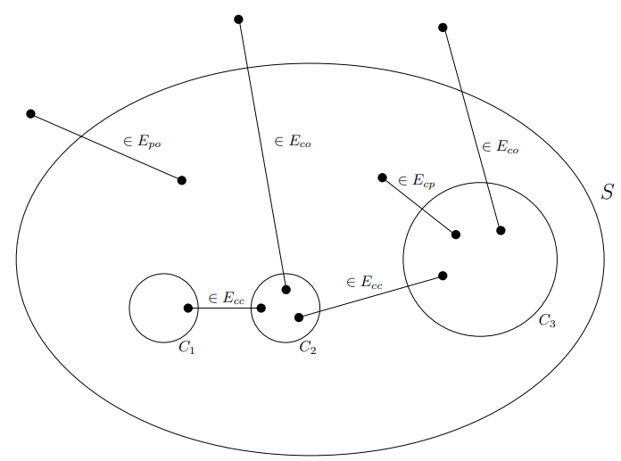
Case 2:SS is an internal nodes with kk children C_(1),C_(2),dots,C_(k)C_{1}, C_{2}, \ldots, C_{k}. See Fig 13.5 for the different types of edges that are relevant. E_(cc)E_{c c} is the set of edges with end points in two different children of SS. E_(cp)E_{c p} be the set of edges that cross exactly one child but do not cross SS. E_(po)E_{p o} be the set of edges that cross SS but do not cross any of the children. E_(co)E_{c o} is the set of edges that cross both a child and SS. This notation is borrowed from [6:1].
Figure 13.5: SS is an internal node with several children. Different types of edges that play a role. pp refers to parent set S,cS, c refer to a child set and oo refers to outside.
Let gamma(S)\gamma(S) be the number of edges whose both endpoints belong to SS but not to any child of SS. Note that gamma(S)=|E_(cc)|+|E_(cp)|\gamma(S)=\left|E_{c c}\right|+\left|E_{c p}\right|.
(13.1) follows by applying the inductive hypothesis to each child. From the preceding inequality, to prove that beta(S) >= alpha(S)-f(S)\beta(S) \geq \alpha(S)-f(S) (the claim for SS), it suffices to show the following inequality.
Case 2.1:gamma(S)=0\gamma(S)=0. This implies that E_(cc)E_{c c} and E_(cp)E_{c p} are empty. Since chi(delta(S))\chi(\delta(S)) is linearly independent from chi(delta(C_(1))),dots,chi(delta(C_(k)))\chi\left(\delta\left(C_{1}\right)\right), \ldots, \chi\left(\delta\left(C_{k}\right)\right), we must have that E_(po)E_{po} is not empty and hence sum_(e inE_(po))x_(e) > 0\sum_{e \in E_{p o}} x_{e}>0. Therefore, in this case,
Since the left hand side is an integer, it follows that sum_(i=1)^(k)f(C_(i))-f(S)+1 <= 0=gamma(S)\sum_{i=1}^{k} f\left(C_{i}\right)-f(S)+1 \leq 0=\gamma(S).
Case 2.2:gamma(S) >= 1\gamma(S) \geq 1. Recall that gamma(S)=|E_(cc)|+|E_(cp)|\gamma(S)=\left|E_{c c}\right|+\left|E_{c p}\right|.
By our assumption that x_(e) < (1)/(2)x_{e}<\frac{1}{2} for each ee, we have sum_(e inE_(cc))2x_(e) < |E_(cc)|\sum_{e \in E_{c c}} 2 x_{e}<\left|E_{c c}\right| if |E_(cc)| > 0\left|E_{c c}\right|>0, and similarly sum_(e inE_(cp))x_(e) < |E_(cp)|//2\sum_{e \in E_{c p}} x_{e}<\left|E_{c p}\right| / 2 if |E_(cp)| > 0\left|E_{c p}\right|>0. Since gamma(S)=|E_(cc)|+|E_(cp)| >= 1\gamma(S)=\left|E_{c c}\right|+\left|E_{c p}\right| \geq 1 we conclude that
Tightness of the analysis: The LP relaxation has an integrality gap of 22 even for the MST problem. Let GG be the cycle on nn vertices with all edge costs equal to 11. Then setting x_(e)=1//2x_{e}=1 / 2 on each edge is feasible and the cost is n//2n / 2 while the MST cost is n-1n-1. Note that the optimum fractional solution here is 1//21 / 2-integral. However, there are more involved examples (see Jain's paper or [4:1]) based on the Petersen graph where the optimum basic feasible solution is not half-integral while there are one or more edges with fractional value at least 1//21 / 2. Jain's iterated rounding algorithm is an unusual algorithm in that the output of the algorithm may not have any discernible structure until it is completely done.
Running time: The strength of the iterated rounding approach is the remarkable approximation guarantees it delivers for various problems. The weakness is the high running time which is due to two reasons. First, one needs a basic feasible solution for the LP–this is typically much more expensive than finding an approximately good feasible solution. Second, the algorithm requires computing an LP solution many times. Finding faster algorithms with comparable approximation guarantees is an open research area.
The source minimal ss-tt mincut in a directed / undirected graph is unique via submodularity and can be found by computing ss-tt maxflow and finding the reachable set from ss in the residual graph. Similarly sink minimal set. ↩︎
Michel X Goemans and David P Williamson. “The primal-dual method for approximation algorithms and its application to network design problems”. In: Approximation algorithms for NP-hard problems (1997), pp. 144–191. ↩︎
Kamal Jain. “A factor 2 approximation algorithm for the generalized Steiner network problem”. In: Combinatorica 21.1 (2001), pp. 39–60. ↩︎
Vijay V Vazirani. Approximation algorithms. Springer Science & Business Media, 2013. ↩︎↩︎
Viswanath Nagarajan, R Ravi, and Mohit Singh. “Simpler analysis of LP extreme points for traveling salesman and survivable network design problems”. In: Operations Research Letters 38.3 (2010), pp. 156–160. ↩︎
David P Williamson and David B Shmoys. The design of approximation algorithms. Cambridge university press, 2011. ↩︎↩︎
Chandra Chekuri and Thapanapong Rukkanchanunt. “A note on iterated rounding for the Survivable Network Design Problem”. In: 1st Symposium on Simplicity in Algorithms (SOSA 2018). Schloss DagstuhlLeibniz-Zentrum fuer Informatik. 2018. ↩︎
Recommended for you
@lapostadialberto
The use of Mathpix OCR with EDICO scientific editor to help blind Students in STEM education
The use of Mathpix OCR with EDICO scientific editor to help blind Students in STEM education
In this tutorial we'll show how Mathpix OCR is helpful to instantly transpose math and science assignments both in braille and speech. We'll use the free EDICO Scientific Editor to demonstrate how a math assignment can be imported using Mathpix technology, and how it can be solved using a Refreshable Braille Display.