Approximation Algorithms: Introduction to Network Design

This is the lecture notes from Chandra Chekuri's CS583 course on Approximation Algorithms. Chapter 10: Introduction to Network Design. You can read Chapter 11: Steiner Forest Problem, here. Chapter 9: Clustering and Facility Location, here.

Chapter 10

(Parts of this chapter are based on previous scribed lecture notes by Nitish Korula and Sungjin Im.)

Network Design is a broad topic that deals with finding a subgraph

H

of a given graph

G = (V, E)

of minimum cost while satisfying certain requirements.

G

represents an existing network or a constraint over where one can build. The subgraph

H

is what we want to select/build. Many natural problems can be viewed this way. For instance the minimum spanning tree (MST) can be viewed as follows: given an undirected graph

G = (V, E)

with edge costs

c : E \to R_{+}

, find the cheapest connected spanning (spanning means that all vertices are included) subgraph of

G

. The fact that a minimal solution is a tree is clear, but the point is that the motivation does not explicitly mention the requirement that the output be a tree.

Connectivity problems are a large part of network design. As we already saw MST is the most basic one and can be solved in polynomial time. The Steiner Tree problem is a generalization where we are given a subset

S

of terminals in an edgeweighted graph

G = (V, E)

and the goal is to find a cheapest connected subgraph that contains all terminals. This is NP-Hard. Traveling Salesman Problem (TSP) and its variants can also be viewed as network design problems. Network design is heavily motivated by real-world problems in telecommunication networks and those problems combine aspects of connectivity and routing and in this context there are several problems related to buy-at-bulk network design, fixed-charge flow problems etc.

Graph theory plays an important role in most network algorithmic questions. The complexity and nature of the problems vary substantially based on whether the graph is undirected or directed. To illustrate this consider the Directed Steiner Tree problem. Here

G = (V, E)

is a directed graph with non-negative edge/arc weights, and we are given a root

r

and a set of terminals

S \subseteq V

. The goal is to find a cheapest subgraph

H

G

such that

r

has a path to each terminal

t \in S

. Note that when

S = V

the problem is the minimum-cost arborescence problem and is solvable in polynomial-time. One can see that Directed Steiner Tree is a generalization of the (undirected) Steiner Tree problem. While Steiner Tree problem admits a constant factor approximation, it is easy to show that Directed Steiner Tree is at least as hard as Set Cover. This immediately implies that it is hard to approximate to within an

Ω (\log | S |)

factor. In fact, substantial technical work has shown that it is in fact harder than Set Cover ^[1], while we only have a quasi-polynomial time algorithm that gives a poly-logarithmic approximation ^[2]. In even slightly more general settings, the directed graph problems get much harder when compared to their undirected graph counterparts. This phenomena is generally true in many graph related problems and hence the literature mostly focuses on undirected graphs. We refer the reader to some surveys on network design ^[3],^[4],^[5].

This chapter will focus on two basic problems which are extensively studied and describe some simple approximation algorithms for them. Pointers are provided for sophisticated results including some very recent ones.

10.1 The Steiner Tree Problem

In the Steiner Tree problem, the input is a graph

G (V, E)

, together with a set of terminals

S \subseteq V

, and a cost

c (e)

for each edge

e \in E

. The goal is to find a minimum-cost tree that connects all terminals, where the cost of a subgraph is the sum of the costs of its edges.

The Steiner Tree problem is NP-Hard, and also APX-Hard ^[6]. The latter means that there is a constant

δ > 1

such that it is NP-Hard to approximate the solution to within a ratio of less than

δ

; it is currently known that it is hard to approximate the Steiner Tree problem to within a ratio of 95/94 ^[7].^[8]

Remark 10.1. If

| S | = 2

(that is, there are only 2 terminals), an optimal Steiner Tree is simply a shortest path between these 2 terminals. If

S = V

(that is, all vertices are terminals), an optimal solution is simply a minimum spanning tree of the input graph. In both these cases, the problem can be solved exactly in polynomial time.

Remark 10.2. There is

c^{k}

poly

(n)

-time algorithm where

k

is the number of terminals. Can you figure it out?

Definition 10.1. Given a connected graph $G (V, E)$ with edge costs, the metric completion of

G

is a complete graph

H (V, E^{'})

such that for each

u, v \in V

, the cost of edge

u v

H

is the cost of the shortest path in

G

from

u

v

. The graph

H

with edge costs is a metric on

V

, because the edge costs satisfy the triangle inequality:

\forall u, v, w, cost (u v) \leq cost (u w) + cost (w v)

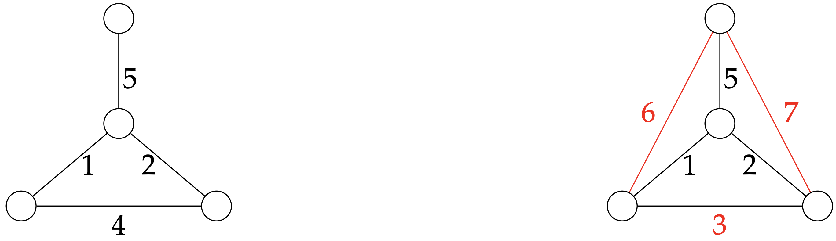
Figure 10.1: On the left, a graph. On the right, its metric completion, with new edges and modified edge costs in red.

Observation 10.2. To solve the Steiner Tree problem on a graph $G$ , it suffices to solve it on the metric completion of $G$ .

We now look at two approximation algorithms for the Steiner Tree problem.

10.1.1 The MST Algorithm

The following algorithm, with an approximation ratio of

(2 - 2 / | S |)

is due to ^[9]:

\underline{SteinerMST (G (V, E), S \subseteq V) :}

Let

H (V, E^{'}) \leftarrow

metric completion of

G .

Let

T \leftarrow

MST of

H [S]

Output

T

(Here, we use the notation

H [S]

to denote the subgraph of

H

induced by the set of terminals

S

The following lemma is central to the analysis of the algorithm SteinerMST.

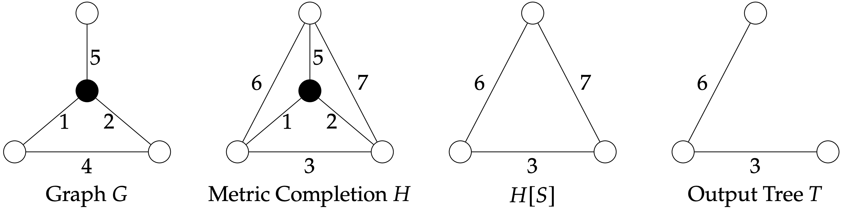
Lemma 10.1. For any instance I of Steiner Tree , let $H$ denote the metric completion of the graph, and $S$ the set of terminals. There exists a spanning tree in $H [S]$ (the graph induced by terminals) of cost at most $2 (1 - \frac{1}{| S |}) OPT$ , where $OPT$ is the cost of an optimal solution to instance I.

Figure 10.2: Illustrating the MST Heuristic for Steiner Tree

Before we prove the lemma, we note that if there exists some spanning tree in

H [S]

of cost at most

2 (1 - \frac{1}{| S |}) OPT

, the minimum spanning tree has at most this cost. Therefore, Lemma 10.1 implies that the algorithm SteinerMST is a

2 (1 - \frac{1}{| S |})

-approximation for the Steiner Tree problem.

Proof. Proof of Lemma 10.1 Let

T^{*}

denote an optimal solution in

H

to the given instance, with

cost c (T^{*})

. Double all the edges of

T^{*}

to obtain an Eulerian graph, and fix an Eulerian Tour

W

of this graph. See Fig 10.3. Now, shortcut edges of

W

to obtain a tour

W^{'}

of the vertices in

T^{*}

in which each vertex is visited exactly once. Again, shortcut edges of

W^{'}

to eliminate all non-terminals; this gives a walk

W^{''}

that visits each terminal exactly once.

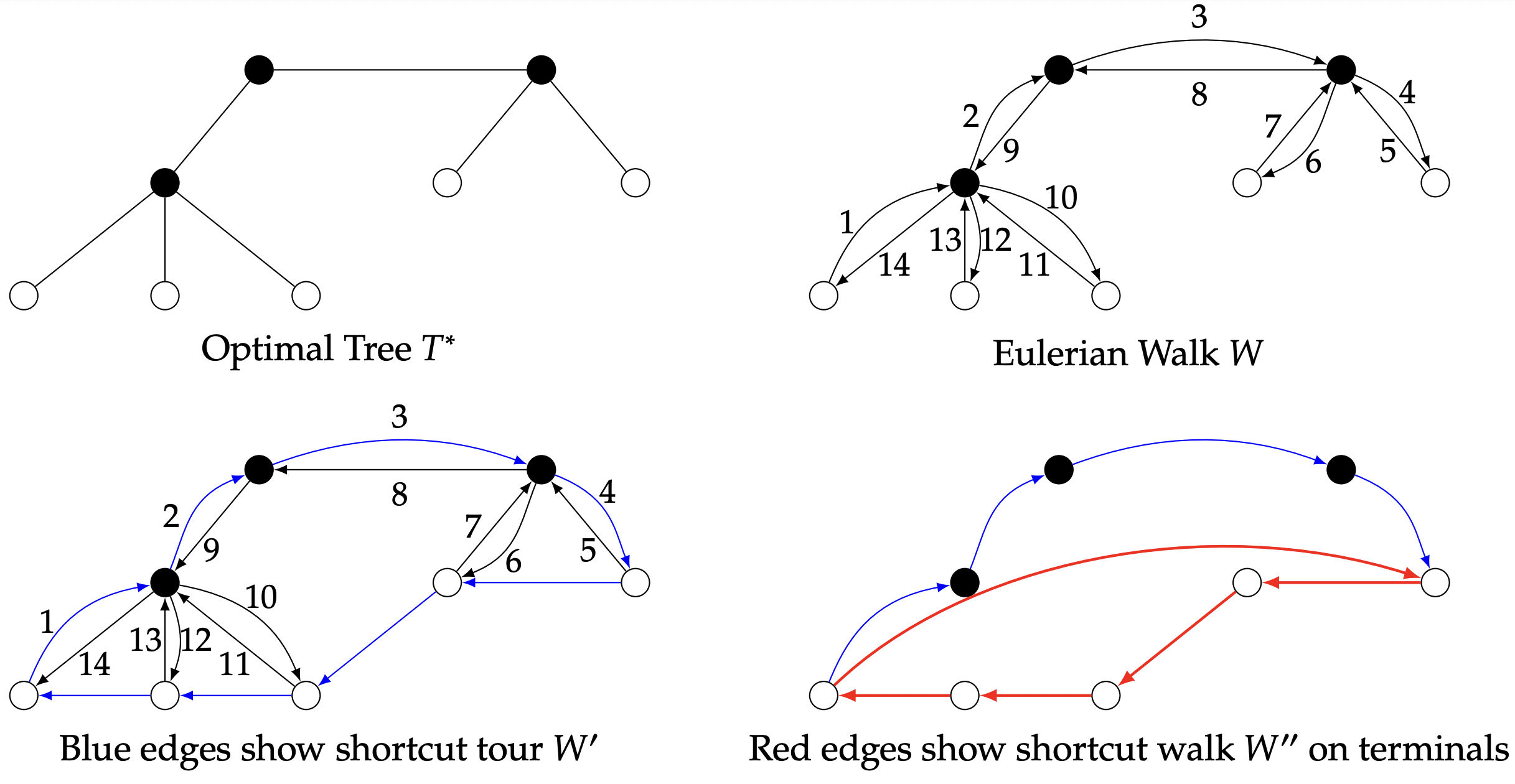
Figure 10.3: Doubling edges of

T^{*}

and shortcutting gives a low-cost spanning tree on terminals.

It is easy to see that

c (W^{''}) \leq c (W^{'}) \leq c (W) = 2 c (T^{*})

, where the inequalities follow from the fact that by shortcutting, we can only decrease the length of the walk. (Recall that we are working in the metric completion

H

.) Now, delete the heaviest edge of

W^{''}

to obtain a path through all the terminals in

S

, of cost at most

(1 - \frac{1}{| S |}) c (W^{''})

. This path is a spanning tree of the terminals, and contains only terminals; therefore, there exists a spanning tree in

H [S]

of cost at most

2 (1 - \frac{1}{| S |}) c (T^{*})

A tight example: The following example (Fig. 4 below) shows that this analysis is tight; there are instances of Steiner Tree where the SteinerMST algorithm finds a tree of

cost 2 (1 - \frac{1}{S})

OPT. Here, each pair of terminals is connected by an edge of cost 2, and each terminal is connected to the central non-terminal by an edge of cost 1. The optimal tree is a star containing the central non-terminal, with edges to all the terminals; it has cost

| S |

. However, the only trees in

H [S]

are formed by taking

| S | - 1

edges of cost 2; they have cost

2 (| S | - 1)

Figure 10.4: A tight example for the SteinerMST algorithm

10.1.2 The Greedy/Online Algorithm

We now describe another simple algorithm for the Steiner Tree problem, due to ^[10].

\underline{GreedySteiner (G (V, E), S \subseteq V) :}

Let

{s_{1}, s_{2}, \dots s_{| S |}}

be an arbitrary ordering of the terminals.

Let

T \leftarrow {s_{1}}

For

(i

from

2

| S |)

Let

P_{i}

be the shortest path in

G

from

s_{i}

T

Add

P_{i}

T

GreedySteiner is a

⌈ \log_{2} | S | ⌉

-approximation algorithm; here, we prove a slightly weaker result.

Theorem 10.3. The algorithm GreedySteiner has an approximation ratio of $2 H_{| S |} \approx$ $2 \ln | S |$ , where $H_{i} = \sum_{j = 1}^{i} 1 / j$ denotes the $i^{'}$ th harmonic number.

Note that this is an online algorithm; terminals are considered in an arbitrary order, and when a terminal is considered, it is immediately connected to the existing tree. Thus, even if the algorithm could not see the entire input at once, but instead terminals were revealed one at a time and the algorithm had to produce a Steiner tree at each stage, the algorithm GreedySteiner outputs a tree of cost no more than

O (\log | S |)

times the cost of the optimal tree.

To prove Theorem 10.3, we introduce some notation. Let

c (i)

denote the cost of the path

P_{i}

used in the

i

th iteration to connect the terminal

s_{i}

to the already existing tree. Clearly, the total cost of the tree is

\sum_{i = 1}^{| S |} c (i)

. Now, let

{i_{1}, i_{2}, \dots i_{| S |}}

be a permutation of

{1, 2, \dots | S |}

such that

c (i_{1}) \geq c (i_{2}) \geq \dots \geq c (i_{| S |})

. (That is, relabel the terminals in decreasing order of the cost paid to connect them to the tree that exists when they are considered by the algorithm.)

Claim 10.1.1. For all $j$ , the cost $c (i_{j})$ is at most $2 OPT / j$ , where $OPT$ is the cost of an optimal solution to the given instance.

Proof. Suppose by way of contradiction this were not true; since

s_{i_{j}}

is the terminal with

j

th highest cost of connection, there must be

j

terminals that each pay more than

2 OPT / j

to connect to the tree that exists when they are considered. Let

S^{'} = {s_{i_{1}}, s_{i_{2}}, \dots s_{i_{j}}}

denote this set of terminals.

We argue that no two terminals in

S^{'} \cup {s_{1}}

are within distance

2 OPT / j

of each other. If some pair

x, y

were within this distance, one of these terminals (say

y

) must be considered later by the algorithm than the other. But then the cost of connecting

y

to the already existing tree (which includes

x

) must be at most

2 OPT / j

, and we have a contradiction.

Therefore, the minimum distance between any two terminals in

S^{'} \cup {s_{1}}

must be greater than

2 OPT / j

. Since there must be

j

edges in any MST of these terminals, an MST must have cost greater than 2 OPT. But the MST of a subset of terminals cannot have cost more than

2 OPT

, exactly as argued in the proof of Lemma 10.1. Therefore, we obtain a contradiction.

Given this claim, it is easy to prove Theorem 10.3.

\sum_{i = 1}^{| S |} c (i) = \sum_{j = 1}^{| S |} c (i_{j}) \leq \sum_{j = 1}^{| S |} \frac{2 OPT}{j} = 2 OPT \sum_{j = 1}^{| S |} \frac{1}{j} = 2 H_{| S |} \cdot OPT .

Question 10.2. Give an example of a graph and an ordering of terminals such that the output of the Greedy algorithm is

Ω (\log | S |) OPT

Remark 10.3. We emphasize again that the analysis above holds for every ordering of the terminals. A natural variant might be to adaptively order the terminals so that in each iteration

i

, the algorithm picks the terminal

s_{i}

to be the one closest to the already existing tree

T

built in the first

i

iterations. Do you see that this is equivalent to using the MST Heuristic with Prim's algorithm for MST? This illustrates the need to be careful in the design and analysis of heuristics.

10.1.3 LP Relaxation

A natural LP relaxation for the Steiner Tree problem is the following. For each edge

e \in E

we have an indicator variable

x_{e}

to decide if we choose to include

e

in our solution. The chosen edges should ensure that no two terminals are separated. We write this via a constraint

\sum_{e \in δ (A)} x_{e} \geq 1

for any set

A \subset V

such that

A

contains a terminal and

V ∖ A

contains a terminal.

\begin{aligned} \sum_{e \in δ (A)}^{min_{e \in E} c_{e} x_{e}} x_{e} & \geq 1 A \cap S \neq \emptyset, (V - A) \cap S \neq \emptyset \\ x_{e} & \geq 0 \end{aligned}

Note that the preceding LP has an exponential number of constraints. However, there is a polynomial-time separation oracle. Given

x

it is feasible for the LP iff the

s - t

cut value is at least

1

between any two terminals

s, t \in S

with edge capacities given by

x

. How good is this LP relaxation? We will see later that there is a

2 (1 - 1 / | S |)

-approximation via this LP. Interestingly the LP has an integrality gap of

2 (1 - 1 / | S |)

even if

S = V

in which case we want to solve the MST problem! Despite the weakness of this cut based LP for these simple cases, we will see later that it generalizes nicely for higher connectivity problems and one can derive a 2-approximation even for those much more difficult problems.

10.1.4 Other Results on Steiner Trees

The 2-approximation algorithm using the MST Heuristic is not the best approximation algorithm for the Steiner Tree problem currently known. Some other results on this problem are listed below.

The first algorithm to obtain a ratio of better than $2$ was due to due to Alexander Zelikovsky ^[11]; the approximation ratio of this algorithm was $11 / 6 \approx 1.83$ . This was improved to $1 + \frac{\ln 3}{2} \approx 1.55$ ^[12] and is based on a local search based improvement starting with the MST heuristic, and follows the original approach of Zelikovsky.
Byrka et al gave an algorithm with an approximation ratio of $1.39 = \ln 4 + ϵ$ ^[13] which is currently the best known for this problem. This was originally based on a combination of techniques and subsequently there is an LP based proof ^[14] that achieves the same approximation for the so-called Hypergraphic LP relaxation.
The bidirected cut LP relaxation for the Steiner Tree was proposed by ^[15]; it has an integrality gap of at most $2 (1 - \frac{1}{| S |})$ , but it is conjectured that the gap is smaller. No algorithm is currently known that exploits this LP relaxation to obtain an approximation ratio better than that of the SteinerMST algorithm. Though the true integrality gap is not known, there are examples that show it is at least $6 / 5 = 1.2$ ^[16].
For many applications, the vertices can be modeled as points on the plane, where the distance between them is simply the Euclidean distance. The MST-based algorithm performs fairly well on such instances; it has an approximation ratio of $2 / \sqrt{3} \approx 1.15$ ^[17]. An example which achieves this bound is three points at the corners of an equilateral triangle, say of side-length 1; the MST heuristic outputs a tree of cost 2 (two sides of the triangle) while the optimum solution is to connect the three points to a Steiner vertex which is the circumcenter of the triangle. One can do better still for instances in the plane (or in any Euclidean space of small-dimensions); for any $ϵ > 0$ , there is a $1 + ϵ$ -approximation algorithm that runs in polynomial time ^[18]. Such an approximation scheme is also known for planar graphs ^[19] and more generally bounded-genus graphs.

10.2 The Traveling Salesperson Problem (TSP)

10.2.1 TSP in Undirected Graphs

In the Traveling Salesperson Problem (TSP), we are given an undirected graph

G = (V, E)

and

cost c (e) > 0

for each edge

e \in E

. Our goal is to find a Hamiltonian cycle with minimum cost. A cycle is said to be Hamiltonian if it visits every vertex in

V

exactly once.

TSP is known to be NP-Hard. Moreover, we cannot hope to find a good approximation algorithm for it unless

P = N P

. This is because if one can give a good approximation solution to TSP in polynomial time, then we can exactly solve the NP-Complete Hamiltonian cycle problem (HAM) in polynomial time, which is not possible unless

P = N P

. Recall that HAM is a decision problem: given a graph

G = (V, E)

, does

G

have a Hamiltonian cycle?

Theorem 10.4 (^[20]). Let $α : N \to N$ be a polynomial-time computable function. Unless $P = N P$ there is no polynomial-time algorithm that on every instance I of TSP outputs a solution of cost at most $α (| I |) \cdot O P T (I)$ .

Proof. For the sake of contradiction, suppose we have an approximation algorithm

A

for TSP with an approximation ratio

α (| I |)

. We show a contradiction by showing that using

A

, we can exactly solve HAM in polynomial time. Let

G = (V, E)

be the given instance of HAM. We create a new graph

H = (V, E^{'})

with cost

c (e)

for each

e \in E^{'}

such that

c (e) = 1

e \in E

, otherwise

c (e) = B

, where

B = n α (n) + 2

and

n = | V |

. Note that this is a polynomial-time reduction since

α

is a polynomial-time computable function.

We observe that if

G

has a Hamiltonian cycle,

OPT = n

, otherwise

OPT \geq

n - 1 + B \geq n α (n) + 1

. (Here, OPT denotes the cost of an optimal TSP solution in

H

.) Note that there is a "gap" between when

G

has a Hamiltonian cycle and when it does not. Thus, if

A

has an approximation ratio of

α (n)

, we can tell whether

G

has a Hamiltonian cycle or not: Simply run

A

on the graph

H

; if

A

returns a TSP tour in

H

of cost at most

α (n) n

output that

G

has a Hamilton cycle, otherwise output that

G

has no Hamilton cycle. We leave it as an exercise to formally verify that this would solve HAM in polynomial time.

Since we cannot even approximate the general TSP problem, we consider more tractable variants.

Metric-TSP: In Metric-TSP, the instance is a complete graph $G = (V, E)$ with cost $c (e)$ on $e \in E$ , where $c$ satisfies the triangle inequality, i.e. $c (u w) \leq c (u v) + c (v w)$ for any $u, v, w \in V$ .
TSP-R: TSP with repetitions of vertices allowed. The input is a graph $G = (V, E)$ with non-negative edge costs as in TSP. Now we seek a minimum-cost walk that visits each vertex at least once and returns to the starting vertex.

Exercise 10.1. Show that an

α

-approximation for Metric-TSP implies an

α

approximation for TSP-R and vice-versa.

We focus on Metric-TSP for the rest of this section. We first consider a natural greedy approach, the Nearest Neighbor Heuristic (NNH).

\underline{Nearest Neighbor Heuristic (G (V, E), c : E \to R^{+}) :}

Start at an arbitrary vertex

s

While (there are unvisited vertices)

From the current vertex

u

, go to the nearest unvisited vertex

v

Return to

s

Exercise 10.2. 1.Prove that NNH is an

O (\log n)

-approximation algorithm. (Hint: Think back to the proof of the

2 H_{| S |}

-approximation for the Greedy Steiner Tree Algorithm.)

NNH is not an $O$ (1)-approximation algorithm; can you find an example to show this? In fact one can show a lower bound of $Ω (\log n)$ on the approximation-ratio achieved by NNH.

There are constant-factor approximation algorithms for TSP; we now consider an MST-based algorithm. See Fig 10.5.

\underline{TSP-MST (G (V, E), c : E \to R^{+}) :}

Compute an MST

T

G

Obtain an Eulerian graph

H = 2 T

by doubling edges of

T

An Eulerian tour of

2 T

gives a tour in

G

Obtain a Hamiltonian cycle by shortcutting the tour.

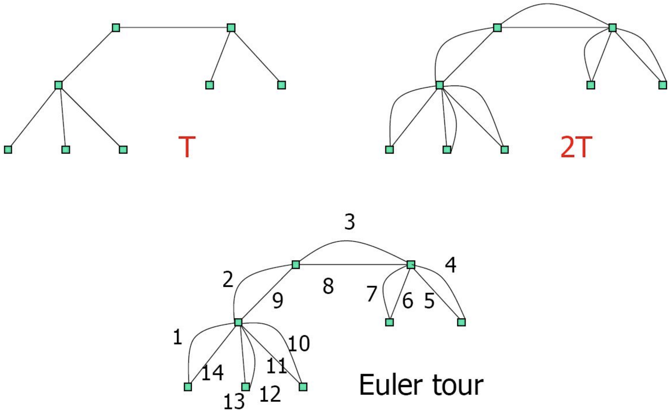
Figure 10.5: MST Based Heuristic

Theorem 10.5. MST heuristic(TSP-MST) is a 2-approximation algorithm.

Proof. We have

c (T) = \sum_{e \in E (T)} c (e) \leq OPT

, since we can get a spanning tree in

G

by removing any edge from the optimal Hamiltonian cycle, and

T

is a MST. Thus

c (H) = 2 c (T) \leq 2 OPT

. Also shortcutting only decreases the cost.

We observe that the loss of a factor 2 in the approximation ratio is due to doubling edges; we did this in order to obtain an Eulerian tour. But any graph in which all vertices have even degree is Eulerian, so one can still get an Eulerian tour by adding edges only between odd degree vertices in

T

. Christofides Heuristic ^[21] exploits this and improves the approximation ratio from

2

3 / 2

. See Fig 10.6 for a snapshot.

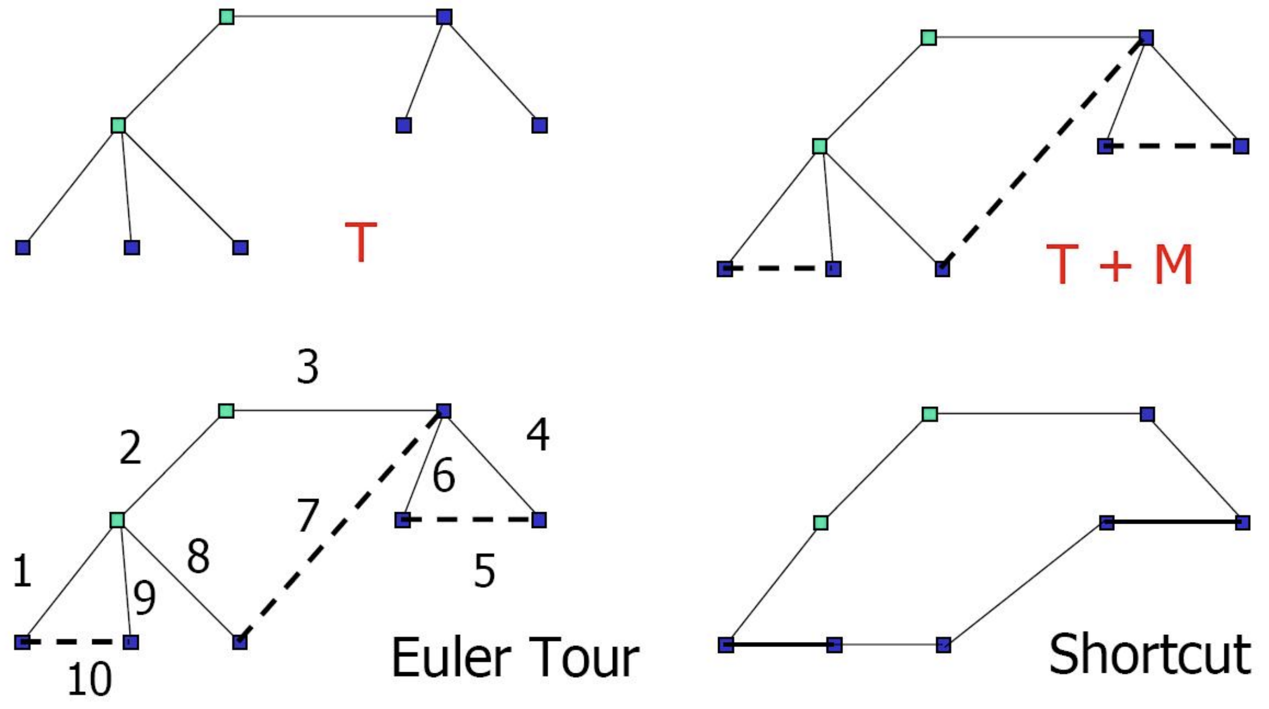
Figure 10.6: Christofides Heuristic

\underline{Christofides Heuristic (G (V, E), c : E \to R^{+}) :}

Compute an MST

T

G

Let

S

be the vertices of odd degree in

T

. (Note:

| S |

is even)

Find a minimum cost matching

M

S

G

Add

M

T

to obtain an Eulerian graph

H

Compute an Eulerian tour of

H

Obtain a Hamilton cycle by shortcutting the tour.

Theorem 10.6. Christofides Heuristic is a 1.5-approximation algorithm.

Proof. The main part of the proof is to show that

c (M) \leq .5 OPT

. Suppose that

c (M) \leq .5 OPT

. Then, since the solution of Christofides Heuristic is obtained by shortcutting the Eulerian tour on

H

, its cost is no more than

c (H) = c (T) + c (M) \leq 1.5 OPT

. (Refer to the proof of Lemma

10.5

for the fact

c (T) \leq OPT

.) Therefore we focus on proving that

c (M) \leq .5 OPT

Let

F^{*}

be an optimal tour in

G

of cost

OPT

; since we have a metric-instance we can assume without loss of generality that

F^{*}

is a Hamiltonian cycle. We obtain a Hamiltonian cycle

F_{S}^{*}

in the graph

G [S]

by short-cutting the portions of

F^{*}

that touch the vertices

V ∖ S

. By the metric-condition,

c (F_{S}^{*}) \leq c (F^{*}) = OPT

. Let

S = {v_{1}, v_{2}, \dots, v_{| S |}}

. Without loss of generality

F_{S}^{*}

visits the vertices of

S

in the order

v_{1}, v_{2}, \dots, v_{| S |}

. Recall that

| S |

is even. Let

M_{1} = {v_{1} v_{2}, v_{3} v_{4}, \dots v_{| S | - 1} v_{| S |}}

and

M_{2} = {v_{2} v_{3}, v_{4} v_{5}, \dots v_{| S |} v_{1}}

. Note that both

M_{1}

and

M_{2}

are matchings, and

c (M_{1}) + c (M_{2}) = c (F_{S}^{*}) \leq OPT

. We can assume without loss of generality that

c (M_{1}) \leq c (M_{2})

. Then we have

c (M_{1}) \leq .5 OPT

. Also we know that

c (M) \leq c (M_{1})

, since

M

is a minimum cost matching on

S

G [S]

. Hence we have

c (M) \leq c (M_{1}) \leq .5 OPT

, which completes the proof.

10.2.2 LP Relaxation

We describe a well-known LP relaxation for TSP called the Subtour-Elimination LP and sometimes also called the Held-Karp LP relaxation although the formulation was first given by Dantzig, Fulkerson and Johnson ^[22]. The LP relaxation has a variable

x_{e}

for each edge

e \in E

. Note that the TSP solution is a Hamilton Cycle of least cost. A Hamilton cycle can be viewed as a connected subgraph of

G

with degree

2

at each vertex. Thus we write the degree constraints and also the cut constraints.

\begin{aligned} min_{e \in E} c_{e} x_{e} \\ \sum_{e \in δ (v)} x_{e} & = 2 v \in V \\ \sum_{e \in δ (S)} x_{e} & \geq 2 \emptyset ⊊ S ⊊ V \\ x_{e} & \in [0, 1] e \in E \end{aligned}

The relaxation is not useful for a general graph since we saw that TSP is not approximable. To obtain a relaxation for Metric-TSP we apply the above to the metric completion of the graph

G

Another alternative is to consider the following LP which view the problem as finding a connected Eulerian multi-graph of the underlying graph

G

. In other words we are allowed to take an integer number of copies of each edge with the constraint that the degree of each vertex is even and the graph is connected. It is not easy to write the even degree condition since we do not have an apriori bound. Instead one can write the following simpler LP, and interestingly one can show that its optimum value is the same as that of the preceding relaxation (when applied to the metric completion).

\begin{aligned} min_{e \in E} c_{e} x_{e} \\ \sum_{e \in δ (S)} x_{e} & \geq 2 \emptyset ⊊ S ⊊ V \\ x_{e} & \in 0 e \in E \end{aligned}

Wolsey showed that the

3 / 2

-approximation of Christofides can be analyzed with respect to the LP above. Hence the integrality gap of the LP is at most

3 / 2

with respect to the LP above. Hence the integrality gap of the LP is at most

3 / 2

for Metric-TSP. Is it better? There is a well-known example which shows that the gap is at least

4 / 3

. The

4 / 3

conjecture states that the worst-case integrality gap very very recently that the

3 / 2

barrier was broken.

Remarks

In practice, local search heuristics are widely used and they perform extremely well. A popular heuristic 2-Opt is to swap pairs from $x y, z w$ to $x z, y w$ or $x w, y z$ , if it improves the tour.
It was a major open problem to improve the approximation ratio of $\frac{3}{2}$ for Metric-TSP; it is conjectured that the Held-Karp LP relaxation ^[23] gives a ratio of $\frac{4}{3}$ . In a breakthrough Oveis-Gharan, Saberi and Singh ^[24] obtained a $3 / 2 - δ$ approximation for some small but fixed $δ > 0$ for the important special case where $c (e) = 1$ for each edge $e$ (called Graphic-TSP). Very recently the $3 / 2$ ratio was finally broken for the general case ^[25].

10.2.3 TSP in Directed Graphs

In this subsection, we consider TSP in directed graphs. As in undirected TSP, we need to relax the problem conditions to get any positive result. Again, allowing each vertex to be visited multiple times is equivalent to imposing the asymmetric triangle inequality

c (u, w) \leq c (u, v) + c (v, w)

for all

u, v, w

. This is called the asymmetric TSP (ATSP) problem. We are given a directed graph

G = (V, A)

with

cost c (a) > 0

for each arc

a \in A

and our goal is to find a closed walk visiting all vertices. Note that we are allowed to visit each vertex multiple times, as we are looking for a walk, not a cycle. For an example of a valid Hamiltonian walk, see Fig 10.7.

The MST-based heuristic for the undirected case has no meaningful generalization to the directed setting This is because costs on edges are not symmetric. Hence, we need another approach. The Cycle Shrinking Algorithm repeatedly finds a min-cost cycle cover and shrinks cycles, combining the cycle covers found. Recall that a cycle cover is a collection of disjoint cycles covering all vertices. It is known that finding a minimum-cost cycle cover can be done in polynomial time (see Homework 0). The Cycle Shrinking Algorithm achieves a

\log_{2} n

approximation ratio.

Figure 10.7: A directed graph and a valid Hamiltonian walk

\underline{Cycle Shrinking Algorithm (G (V, E), c : E \to R^{+}) :}

Transform

G

s.t.

G

is complete and satisfies

c (u, v) + c (v, w) \geq c (u, w)

for

\forall u, v, w

| V | = 1

output the trivial cycle consisting of the single node

Find a minimum cost cycle cover with cycles

C_{1}, \dots, C_{k}

From each

C_{i}

pick an arbitrary proxy node

v_{i}

Recursively solve problem on

G [{v_{1}, \dots, v_{k}}]

to obtain a solution

C

C^{'} = C \cup C_{1} \cup C_{2} \dots C_{k}

is a Eulerian graph.

Shortcut

C^{'}

to obtain a cycle on

V

and output

C^{'}

For a snapshot of the Cycle Shrinking Algorithm, see Fig 10.8.

Figure 10.8: A snapshot of Cycle Shrinking Algorithm. To the left, a cycle cover

C_{1}

. In the center, blue vertices indicate proxy nodes, and a cycle cover

C_{2}

is found on the proxy nodes. To the right, pink vertices are new proxy nodes, and a cycle cover

C_{3}

is found on the new proxy nodes.

Lemma 10.3. Let the cost of edges in $G$ satisfy the asymmetric triangle inequality. Then for any $S \subseteq V$ , the cost of an optimal TSP tour in $G [S]$ is at most the cost of an optimal TSP tour in

G

Proof. Since

G

satisfies the triangle inequality there is an optimal tour TSP tour in

G

that is a Hamiltonian cycle

C

. Given any

S \subseteq V

the cycle

C

can be short-cut to produce another cycle

C^{'}

that visits only

S

and whose cost is at most the cost of

C

Lemma 10.4. The cost of a min-cost cycle-cover is at most the cost of an optimal TSP tour.

Proof. An optimal TSP tour is a cycle cover.

Theorem 10.7. The Cycle Shrinking Algorithm is a $\log_{2} n$ -approximation for ATSP.

Proof. We prove the above by induction on

n

the number of nodes in

G

. It is easy to see that the algorithm finds an optimal solution if

n \leq 2

. The main observation is that the number of cycles in the cycle-cover is at most

⌊ n / 2 ⌋

; this follows from the fact that each cycle in the cover has to have at least 2 nodes and they are disjoint. Thus

k \leq ⌊ n / 2 ⌋

. Let

OPT (S)

denote the cost of an optimal solution in

G [S]

. From Lemma 10.3 we have that

OPT (S) \leq OPT (V) = OPT

for all

S \subseteq V

. The algorithm recurses on the proxy nodes

S = {v_{1}, \dots, v_{k}}

. Note that

| S | < n

, and by induction, the cost of the cycle

C

output by the recursive call is at most

(\log_{2} | S |) OPT (S) \leq (\log_{2} | S |) OPT

The algorithm outputs

C^{'}

whose cost is at most the cost of

C

plus the cost of the cycle-cover computed in

G

. The cost of the cycle cover is at most

OPT

(Lemma 10.4). Hence the cost of

C^{'}

is at most

(\log_{2} | S |) OPT + OPT \leq (\log_{2} n / 2) OPT + OPT \leq (\log_{2} n) OPT

; this finishes the inductive proof.

10.2.4 LP Relaxation

The LP relaxation for ATSP is given below. For each arc

e \in E

we have a variable

x_{e}

. We view the problem as finding a connected Eulerian multi-graph in the support of

G

. That is, we can choose each edge

e

an integer number of times. We impose Eulerian constraint at each vertex by requiring the in-degree to be equal to the out-degree. We impose connectivity constraint by ensuring that at least one arc leaves each set of vertices

S

which is not

V

\emptyset

\begin{aligned} min_{e \in E} c_{e} x_{e} \\ \sum_{e \in δ^{+} (v)} x_{e} - \sum_{e \in δ^{-} (v)} x_{e} & = 0 v \in V \\ \sum_{e \in δ^{+} (S)} x_{e} & \geq 1 \emptyset ⊊ S ⊊ V \\ x_{e} & \geq 0 e \in E \end{aligned}

Remarks:

It has remained an open problem for more than 25 years whether there exists a constant factor approximation for ATSP. Asadpour et al ^[26] have obtained an $O (\log n / \log \log n)$ -approximation for ATSP using some very novel ideas and a well-known LP relaxation.
There is now an $O$ (1)-approximation for ATSP with initial breakthrough work by Svensson for a special case ^[27] and then followed up by Svensson, Tarnawski and Vegh ^[28] . The current best constant is $22 + ϵ$ due to ^[29]. The algorithm is highly non-trivial and is based on the LP relaxation.

Eran Halperin and Robert Krauthgamer. “Polylogarithmic inapproximability”. In: Proceedings of the thirty-fifth annual ACM symposium on Theory of computing. 2003, pp. 585–594. ↩︎
Moses Charikar, Chandra Chekuri, To-Yat Cheung, Zuo Dai, Ashish Goel, Sudipto Guha, and Ming Li. “Approximation algorithms for directed Steiner problems”. In: Journal of Algorithms 33.1 (1999), pp. 73–91. ↩︎
Anupam Gupta and Jochen Könemann. “Approximation algorithms for network design: A survey”. In: Surveys in Operations Research and Management Science 16.1 (2011), pp. 3–20. ↩︎
Guy Kortsarz and Zeev Nutov. “Approximating minimum cost connectivity problems”. In: Parameterized complexity and approximation algorithms. Ed. by Erik D. Demaine, MohammadTaghi Hajiaghayi, and Dániel Marx. Dagstuhl Seminar Proceedings 09511. Dagstuhl, Germany: Schloss Dagstuhl - Leibniz-Zentrum fuer Informatik, Germany, 2010. url: http://drops.dagstuhl.de/opus/volltexte/2010/2497. ↩︎
Zeev Nutov. “Node-connectivity survivable network problems”. In: Handbook of Approximation Algorithms and Metaheuristics. Chapman and Hall/CRC, 2018, pp. 233–253. ↩︎
Marshall Bern and Paul Plassmann. “The Steiner problem with edge lengths 1 and 2”. In: Information Processing Letters 32.4 (1989), pp. 171–176. ↩︎
Miroslav Chlebık and Janka Chlebıková. “Approximation hardness of the Steiner tree problem on graphs”. In: Scandinavian Workshop on Algorithm Theory. Springer. 2002, pp. 170–179. ↩︎
Variants of the Steiner Tree problem, named after Jakob Steiner, have been studied by Fermat, Weber, and others for centuries. The front cover of the course textbook contains a reproduction of a letter from Gauss to Schumacher on a Steiner tree question. ↩︎
Hiromitsu Takahashi and A Matsuyama. “An approximate solution for the Steiner problem in graphs”. In: Math. Jap. 24.6 (1980), pp. 573–577. ↩︎
Makoto Imase and Bernard M Waxman. “Dynamic Steiner tree problem”. In: SIAM Journal on Discrete Mathematics 4.3 (1991), pp. 369–384. ↩︎
Alexander Z Zelikovsky. “An 11/6-approximation algorithm for the network Steiner problem”. In: Algorithmica 9.5 (1993), pp. 463–470. ↩︎
Gabriel Robins and Alexander Zelikovsky. “Tighter bounds for graph Steiner tree approximation”. In: SIAM Journal on Discrete Mathematics 19.1 (2005), pp. 122–134 ↩︎
Jaroslaw Byrka, Fabrizio Grandoni, Thomas Rothvoß, and Laura Sanita. “An improved LP-based approximation for Steiner tree”. In: Proceedings of the forty-second ACM symposium on Theory of computing. 2010, pp. 583–592. ↩︎
Michel X Goemans, Neil Olver, Thomas Rothvoß, and Rico Zenklusen. “Matroids and integrality gaps for hypergraphic steiner tree relaxations”. In: Proceedings of the forty-fourth annual ACM symposium on Theory of computing. 2012, pp. 1161–1176. ↩︎
Jack Edmonds. “Optimum branchings”. In: Journal of Research of the National Bureau of Standards, B 71 (1967), pp. 233–240. ↩︎
Robert Vicari. “Simplex based Steiner tree instances yield large integrality gaps for the bidirected cut relaxation”. In: arXiv preprint arXiv:2002.07912 (2020). ↩︎
D-Z Du and Frank K. Hwang. “A proof of the Gilbert-Pollak conjecture on the Steiner ratio”. In: Algorithmica 7.1 (1992), pp. 121–135. ↩︎
Sanjeev Arora. “Polynomial time approximation schemes for Euclidean traveling salesman and other geometric problems”. In: Journal of the ACM (JACM) 45.5 (1998), pp. 753–782. ↩︎
Glencora Borradaile, Philip Klein, and Claire Mathieu. “An $O (n \log n)$ approximation scheme for Steiner tree in planar graphs”. In: ACM Transactions on Algorithms (TALG) 5.3 (2009), pp. 1–31. ↩︎
Sartaj Sahni and Teofilo Gonzalez. “P-complete approximation problems”. In: Journal of the ACM (JACM) 23.3 (1976), pp. 555–565. ↩︎
Nicos Christofides. Worst-case analysis of a new heuristic for the travelling salesman problem. Tech. rep. Carnegie-Mellon Univ Pittsburgh Pa Management Sciences Research Group, 1976. ↩︎
George Dantzig, Ray Fulkerson, and Selmer Johnson. “Solution of a largescale traveling-salesman problem”. In: Journal of the operations research society of America 2.4 (1954), pp. 393–410. ↩︎
Michael Held and Richard M Karp. “The traveling-salesman problem and minimum spanning trees”. In: Operations Research 18.6 (1970), pp. 1138–1162. ↩︎
Shayan Oveis Gharan, Amin Saberi, and Mohit Singh. “A randomized rounding approach to the traveling salesman problem”. In: 2011 IEEE 52nd Annual Symposium on Foundations of Computer Science. IEEE. 2011, pp. 550–559. ↩︎
Anna R Karlin, Nathan Klein, and Shayan Oveis Gharan. “A (slightly) improved approximation algorithm for metric TSP”. In: Proceedings of the 53rd Annual ACM SIGACT Symposium on Theory of Computing. 2021, pp. 32–45. ↩︎
Arash Asadpour, Michel X Goemans, Aleksander M ˛adry, Shayan Oveis Gharan, and Amin Saberi. “An O (log n/log log n)-approximation algorithm for the asymmetric traveling salesman problem”. In: Operations Research 65.4 (2017). Preliminary version in Proc. of ACM-SIAM SODA, 2010., pp. 1043–1061. ↩︎
Ola Svensson. “Approximating ATSP by relaxing connectivity”. In: 2015 IEEE 56th Annual Symposium on Foundations of Computer Science. IEEE. 2015, pp. 1–19. ↩︎
Ola Svensson, Jakub Tarnawski, and László A Végh. “A constant-factor approximation algorithm for the asymmetric traveling salesman problem”. In: Journal of the ACM (JACM) 67.6 (2020), pp. 1–53. ↩︎
Vera Traub and Jens Vygen. “An improved approximation algorithm for ATSP”. In: Proceedings of the 52nd Annual ACM SIGACT Symposium on Theory of Computing. 2020, pp. 1–13. ↩︎

Approximation Algorithms: Introduction to Network Design

10.1 The Steiner Tree Problem

10.1.1 The MST Algorithm

10.1.2 The Greedy/Online Algorithm

10.1.3 LP Relaxation

10.1.4 Other Results on Steiner Trees

10.2 The Traveling Salesperson Problem (TSP)

10.2.1 TSP in Undirected Graphs

10.2.2 LP Relaxation

10.2.3 TSP in Directed Graphs

10.2.4 LP Relaxation

Recommended for you

Report Article