Approximation Algorithms: Unrelated Machine Scheduling and Generalized Assignment

This is the lecture notes from Chandra Chekuri's CS583 course on Approximation Algorithms. Chapter 6: Unrelated Machine Scheduling and Generalized Assignment. You can read Chapter 7: Congestion Minimization in Networks, here. Chapter 5: Load Balancing and Bin Packing, here.
Chapter 6
This chapter is based on notes first scribed by Alina Ene.

6.1 Scheduling on Unrelated Parallel Machines

We have a set J J JJ of n n nn jobs, and a set M M MM of m m mm machines. The processing time of job i i ii is p i j p i j p_(ij)p_{i j} on machine j j jj. Let f : J M f : J M f:J rarr Mf: J \rightarrow M be a function that assigns each job to exactly one machine. The makespan of f f ff is max 1 j m i : f ( i ) = j p i j max 1 j m i : f ( i ) = j p i j max_(1 <= j <= m)sum_(i:f(i)=j)p_(ij)\max _{1 \leq j \leq m} \sum_{i: f(i)=j} p_{i j}, where i : f ( i ) = j p i j i : f ( i ) = j p i j sum_(i:f(i)=j)p_(ij)\sum_{i: f(i)=j} p_{i j} is the total processing time of the jobs that are assigned to machine j j jj. In the Scheduling on Unrelated Parallel Machines problem, the goal is to find an assignment of jobs to machines of minimum makespan.
We can write an LP for the problem that is very similar to the routing LP from the previous lecture. For each job i i ii and each machine j j jj, we have a variable x i j x i j x_(ij)x_{i j} that denotes whether job i i ii is assigned to machine j j jj. We also have a variable λ λ lambda\lambda for the makespan. We have a constraint for each job that ensures that the job is assigned to some machine, and we have a constraint for each machine that ensures that the total processing time of jobs assigned to the machines is at most the makespan λ λ lambda\lambda.
minimize λ subject to j M x i j = 1 i J i J x i j p i j λ j M x i j 0 i J , j M minimize λ subject to j M x i j = 1 i J i J x i j p i j λ j M x i j 0 i J , j M {:["minimize"qquadlambda],["subject to"qquadsum_(j in M)x_(ij)=1qquadqquadqquadAA i in J],[sum_(i in J)x_(ij)p_(ij) <= lambdaAA j in M],[x_(ij) >= 0AA i in J","j in M]:}\begin{aligned} \text{minimize}\qquad& \lambda & \\ \text{subject to} \qquad& \sum_{j \in M} x_{i j}=1\qquad\qquad\qquad& \forall i \in J \\ & \sum_{i \in J} x_{i j} p_{i j} \leq \lambda & \forall j \in M \\ &x_{ij}\geq 0 & \forall i \in J, j \in M \end{aligned}
The above LP is very natural, but unfortunately it has unbounded integrality gap. Suppose that we have a single job that has processing time T T TT on each of the machines. Clearly, the optimal schedule has makespan T T TT. However, the LP can schedule the job to the extend of 1 / m 1 / m 1//m1 / m on each of the machines, i.e., it can set x 1 j = 1 / m x 1 j = 1 / m x_(1j)=1//mx_{1 j}=1 / m for all j j jj, and the makespan of the resulting fractional schedule is only T / m T / m T//mT / m.
To overcome this difficulty, we modify the LP slightly. Suppose we knew that the makespan of the optimal solution is equal to λ λ lambda\lambda, where λ λ lambda\lambda is some fixed number. If the processing time p i j p i j p_(ij)p_{i j} of job i i ii on machine j j jj is greater than λ λ lambda\lambda, job i i ii is not scheduled on machine j j jj, and we can strengthen the LP by setting x i j x i j x_(ij)x_{i j} to 0 or equivalently, by removing the variable. More precisely, let S λ = { ( i , j ) i J , j M , p i j λ } S λ = ( i , j ) i J , j M , p i j λ S_(lambda)={(i,j)∣i in J,j in M,p_(ij) <= lambda}\mathcal{S}_{\lambda}=\left\{(i, j) \mid i \in J, j \in M, p_{i j} \leq \lambda\right\}. Given a value λ λ lambda\lambda, we can write the following LP for the problem.
L P ( λ ) _ j : ( i , j ) S λ x i j = 1 i J i : ( i , j ) S λ x i j p i j λ j M x i j 0 ( i , j ) S λ L P ( λ ) _ j : ( i , j ) S λ x i j = 1 i J i : ( i , j ) S λ x i j p i j λ j M x i j 0 ( i , j ) S λ {:[LP(lambda)_],[sum_(j:(i,j)inS_(lambda))x_(ij)=1AA i in J],[sum_(i:(i,j)inS_(lambda))x_(ij)p_(ij) <= lambdaAA j in M],[x_(ij) >= 0qquadqquadqquad AA(i","j)inS_(lambda)]:}\begin{aligned} \underline{\mathbf{LP}(\lambda)}&\\ &\sum_{j:(i, j) \in \mathcal{S}_{\lambda}} x_{i j}=1 &\forall i \in J\\ &\sum_{i:(i, j) \in \mathcal{S}_{\lambda}} x_{i j} p_{i j} \leq \lambda &\forall j \in M\\ &x_{i j} \geq 0&\qquad\qquad\qquad\forall(i, j) \in \mathcal{S}_{\lambda} \end{aligned}
Note that the LP above does not have an objective function. In the following, we are only interested in whether the LP is feasible, i.e, whether there is an assignment that satisfies all the constraints. Also, we can think of λ λ lambda\lambda as a parameter and L P ( λ ) L P ( λ ) LP(lambda)\mathbf{LP}(\lambda) as a family of LPs, one for each value of the parameter. A useful observation is that, if λ λ lambda\lambda is a lower bound on the makespan of the optimal schedule, L P ( λ ) L P ( λ ) LP(lambda)\mathbf{LP}(\lambda) is feasible and it is a valid relaxation for the Scheduling on Unrelated Parallel Machines problem.
Lemma 6.1. Let λ λ lambda^(**)\lambda^{*} be the minimum value of the parameter λ λ lambda\lambda such that L P ( λ ) L P ( λ ) LP(lambda)\mathbf{LP}(\lambda) is feasible. We can find λ λ lambda^(**)\lambda^{*} in polynomial time.
Proof. For any fixed value of λ λ lambda\lambda, we can check whether L P ( λ ) L P ( λ ) LP(lambda)\mathbf{L P}(\lambda) is feasible using a polynomial-time algorithm for solving LPs. Thus we can find λ λ lambda^(**)\lambda^{*} using binary search starting with the interval [ 0 , i , j p i j ] [ 0 , i , j p i j ] [0,sum_(i,j)p_(ij)][0, \sum_{i, j} p_{i j}].
In the following, we will show how to round a solution to L P ( λ ) L P λ LP(lambda^(**))\mathbf{L P}\left(\lambda^{*}\right) in order to get a schedule with makespan at most 2 λ 2 λ 2lambda^(**)2 \lambda^{*}. As we will see shortly, it will help to round a solution to L P ( λ ) L P λ LP(lambda^(**))\mathbf{LP}\left(\lambda^{*}\right) that is a vertex solution.
Let x x xx be a vertex solution to L P ( λ ) L P λ LP(lambda^(**))\mathbf{LP}\left(\lambda^{*}\right). Let G G GG be a bipartite graph on the vertex set J M J M J uu MJ \cup M that has an edge i j i j iji j for each variable x i j 0 x i j 0 x_(ij)!=0x_{i j} \neq 0. We say that job i i ii is fractionally set if x i j ( 0 , 1 ) x i j ( 0 , 1 ) x_(ij)in(0,1)x_{i j} \in(0,1) for some j j jj. Let F F FF be the set of all jobs that are fractionally set, and let H H HH be a bipartite graph on the vertex set F M F M F uu MF \cup M that has an edge i j i j iji j for each variable x i j ( 0 , 1 ) x i j ( 0 , 1 ) x_(ij)in(0,1)x_{i j} \in(0,1); note that H H HH is the induced subgraph of G G GG on F M F M F uu MF \cup M. As shown in Lemma 6.2, the graph H H HH has a matching that matches every job in F F FF to a machine, and we will it in the rounding algorithm.
Lemma 6.2. The graph G G GG has a matching that matches every job in F F FF to a machine.
We are now ready to give the rounding algorithm.
SUPM-Rounding
quad\quad Find λ λ lambda^(**)\lambda^{*}
quad\quad Find a vertex solution x x xx to L P ( λ ) L P λ LP(lambda^(**))\mathbf{L P}\left(\lambda^{*}\right)
quad\quad For each i i ii and j j jj such that x i j = 1 x i j = 1 x_(ij)=1x_{i j}=1, assign job i i ii to machine j j jj
quad\quad Construct the graph H H HH
quad\quad Find a maximum matching M M M\mathcal{M} in H H HH
quad\quad Assign the fractionally set jobs according to the matching M M M\mathcal{M}
Theorem 6.1. Consider the assignment constructed by SUPM-Rounding. Each job is assigned to a machine, and the makespan of the schedule is at most 2 λ 2 λ 2lambda^(**)2 \lambda^{*}.
Proof. By Lemma 6.2, the matching M M M\mathcal{M} matches every fractionally set job to a machine and therefore all of the jobs are assigned. After assigning all of the integrally set jobs, the makespan (of the partial schedule) is at most λ λ lambda^(**)\lambda^{*}. Since M M M\mathcal{M} is a matching, each machine receives at most one additional job. Let i i ii be a fractionally set job, and suppose that i i ii is matched (in M M M\mathcal{M} ) to machine j j jj. Since the pair ( i , j ) ( i , j ) (i,j)(i, j) is in S λ S λ S_(lambda^(**))\mathcal{S}_{\lambda^{*}}, the processing time p i j p i j p_(ij)p_{i j} is at most λ λ lambda^(**)\lambda^{*}, and therefore the total processing time of machine j j jj increases by at most λ λ lambda\lambda after assigning the fractionally set jobs. Therefore the makespan of the final schedule is at most 2 λ 2 λ 2lambda^(**)2 \lambda^{*}.
Exercise 6.1. Give an example that shows that Theorem 6.1 is tight. That is, give an instance and a vertex solution such that the makespan of the schedule SUPM-Rounding is at least ( 2 o ( 1 ) ) λ ( 2 o ( 1 ) ) λ (2-o(1))lambda^(**)(2-o(1)) \lambda^{*}.
Since λ λ lambda^(**)\lambda^{*} is a lower bound on the makespan of the optimal schedule, we get the following corollary.
Corollary 6.2. SUPM-Rounding achieves a 2 2 22-approximation.
Now we turn our attention to Lemma 6.2 and some other properties of vertex solutions to L P ( λ ) L P ( λ ) LP(lambda)\mathbf{L P}(\lambda). The following can be derived from the rank lemma which is described in Chapter A. Here we give a self-contained proof.
Lemma 6.3. If L P ( λ ) L P ( λ ) LP(lambda)\boldsymbol{LP}(\lambda) is feasible, any vertex solution has at most m + n m + n m+nm+n non-zero variables and it sets at least n m n m n-mn-m of the jobs integrally.
Proof. Let x x xx be a vertex solution to L P ( λ ) L P ( λ ) LP(lambda)\mathbf{L P}(\lambda). Let r r rr denote the number of pairs in S λ S λ S_(lambda)\mathcal{S}_{\lambda}. Note that L P ( λ ) L P ( λ ) LP(lambda)\mathbf{LP}(\lambda) has r r rr variables, one for each pair ( i , j ) S λ ( i , j ) S λ (i,j)inS_(lambda)(i, j) \in \mathcal{S}_{\lambda}. If x x xx is a vertex solution, it satisfies r r rr of the constraints of L P ( λ ) L P ( λ ) LP(lambda)\mathbf{LP}(\lambda) with equality. The first set of constraints consists of n n nn constraints, and the second set of constraints consists of m m mm constraints. Therefore at least r ( m + n ) r ( m + n ) r-(m+n)r-(m+n) of the tight constraints are from the third set of constraints, i.e., at least r ( m + n ) r ( m + n ) r-(m+n)r-(m+n) of the variables are set to zero.
We say that job i i ii is set fractionally if x i j ( 0 , 1 ) x i j ( 0 , 1 ) x_(ij)in(0,1)x_{i j} \in(0,1) for some j j jj; job i i ii is set integrally if x i j { 0 , 1 } x i j { 0 , 1 } x_(ij)in{0,1}x_{i j} \in\{0,1\} for all j j jj. Let I I II and F F FF be the set of jobs that are set integrally and fractionally (respectively). Clearly, | I | + | F | = n | I | + | F | = n |I|+|F|=n|I|+|F|=n. Any job i i ii that is fractionally set is assigned (fractionally) to at least two machines, i.e., there exist j j j!=ℓj \neq \ell such that x i j ( 0 , 1 ) x i j ( 0 , 1 ) x_(ij)in(0,1)x_{i j} \in(0,1) and x i ( 0 , 1 ) x i ( 0 , 1 ) x_(iℓ)in(0,1)x_{i \ell} \in(0,1). Therefore there are at least 2 | F | 2 | F | 2|F|2|F| distinct non-zero variables corresponding to jobs that are fractionally set. Additionally, for each job i i ii that is integrally set, there is a variable x i j x i j x_(ij)x_{i j} that is non-zero. Thus the number of non-zero variables is at least | I | + 2 | F | | I | + 2 | F | |I|+2|F||I|+2|F|. Hence | I | + | F | = n | I | + | F | = n |I|+|F|=n|I|+|F|=n and | I | + 2 | F | m + n | I | + 2 | F | m + n |I|+2|F| <= m+n|I|+2|F| \leq m+n, which give us that | I | | I | |I||I| is at least n m n m n-mn-m.
Definition 6.3. A connected graph is a pseudo-tree if the number of edges is at most the number of vertices. A graph is a pseudo-forest if each of its connected components is a pseudo-tree.
Lemma 6.4. The graph G G GG is a pseudo-forest.
Proof. Let C C CC be a connected component of G G GG. We restrict L P ( λ ) L P ( λ ) LP(lambda)\mathbf{L P}(\lambda) and x x xx to the jobs and machines in C C CC to get L P ( λ ) L P ( λ ) LP^(')(lambda)\mathbf{L P}^{\prime}(\lambda) and x x x^(')x^{\prime}. Note that x x x^(')x^{\prime} is a feasible solution to L P ( λ ) L P ( λ ) LP^(')(lambda)\mathbf{L P}^{\prime}(\lambda). Additionally, x x x^(')x^{\prime} is a vertex solution to L P ( λ ) L P ( λ ) LP^(')(lambda)\mathbf{L P}^{\prime}(\lambda). If not, x x x^(')x^{\prime} is a convex combination of two feasible solutions x 1 x 1 x_(1)^(')x_{1}^{\prime} and x 2 x 2 x_(2)^(')x_{2}^{\prime} to L P ( λ ) L P ( λ ) LP^(')(lambda)\mathbf{L P}^{\prime}(\lambda). We can extend x 1 x 1 x_(1)^(')x_{1}^{\prime} and x 2 x 2 x_(2)^(')x_{2}^{\prime} to two solutions x 1 x 1 x_(1)x_{1} and x 2 x 2 x_(2)x_{2} to L P ( λ ) L P ( λ ) LP(lambda)\mathbf{LP}(\lambda) using the entries of x x xx that are not in x x x^(')x^{\prime}. By construction, x 1 x 1 x_(1)x_{1} and x 2 x 2 x_(2)x_{2} are feasible solutions to L P ( λ ) L P ( λ ) LP(lambda)\mathbf{L P}(\lambda). Additionally, x x xx is a convex combination of x 1 x 1 x_(1)x_{1} and x 2 x 2 x_(2)x_{2}, which contradicts the fact that x x xx is a vertex solution. Thus x x x^(')x^{\prime} is a vertex solution to L P ( λ ) L P ( λ ) LP^(')(lambda)\mathbf{LP}^{\prime}(\lambda) and, by Lemma 6.3, x x x^(')x^{\prime} has at most n + m n + m n^(')+m^(')n^{\prime}+m^{\prime} non-zero variables, where n n n^(')n^{\prime} and m m m^(')m^{\prime} are the number of jobs and machines in C C CC. Thus C C CC has n + m n + m n^(')+m^(')n^{\prime}+m^{\prime} vertices and at most n + m n + m n^(')+m^(')n^{\prime}+m^{\prime} edges, and therefore it is a pseudo-tree.
Proof. of Lemma 6.2 Note that each job that is integrally set has degree one in G G GG. We remove each integrally set job from G G GG; note that the resulting graph is H H HH. Since we removed an equal number of vertices and edges from G G GG, it follows that H H HH is a pseudo-forest as well. Now we construct a matching M M M\mathcal{M} as follows.
Note that every job vertex has degree at least 2, since the job is fractionally assigned to at least two machines. Thus all of the leaves (degree-one vertices) of H H HH are machines. While H H HH has at least one leaf, we add the edge incident to the leaf to the matching and we remove both of its endpoints from the graph. If H H HH does not have any leaves, H H HH is a collection of vertex-disjoint cycles, since it is a pseudo-forest. Moreover, each cycle has even length, since H H HH is bipartite. We construct a perfect matching for each cycle (by taking alternate edges), and we add it to our matching.
Exercise 6.2. (Exercise 17.1 17.1 17.117.1 in [1]) Give a proof of Lemma 6.2 using Hall's theorem.

6.2 Generalized Assignment Problem

The Generalized Assignment problem is a generalization of the Scheduling on Unrelated Parallel Machines problem in which there are costs associated with each job-machine pair, in addition to a processing time. More precisely, we have a set J J JJ of n n nn jobs, a set M M MM of m m mm machines, and a target λ λ lambda\lambda. The processing time of job i i ii is p i j p i j p_(ij)p_{i j} on machine j j jj, and the cost of assigning job i i ii to machine j j jj is c i j c i j c_(ij)c_{i j}. Let f : J M f : J M f:J rarr Mf: J \rightarrow M be a function that assigns each job to exactly one machine. The assignment f f ff is feasible if its makespan is at most λ λ lambda\lambda (recall that λ λ lambda\lambda is part of the input), and its cost is i c i f ( i ) i c i f ( i ) sum_(i)c_(if(i))\sum_{i} c_{i f(i)}. In the Generalized Assignment problem, the goal is to construct a minimum cost assignment f f ff that is feasible, provided that there is a feasible assignment.
Remark 6.1. We could allow each machine M j M j M_(j)M_{j} to have a different capacity c j c j c_(j)c_{j} which is more natural in certain settings. However, since p i j p i j p_(ij)p_{i j} values are allowed to depend on j j jj we can scale them to ensure that c j = λ c j = λ c_(j)=lambdac_{j}=\lambda for every j j jj without loss of generality.
In the following, we will show that, if there is an assignment of cost C C CC and makespan at most λ λ lambda\lambda, then we can construct a schedule of cost at most C C CC and makespan at most 2 λ 2 λ 2lambda2 \lambda. In fact the assignment will have a stronger property that the load on a a machine exceeds λ λ lambda\lambda due to at most one job.
As before, we let S λ S λ S_(lambda)\mathcal{S}_{\lambda} denote the set of all pairs ( i , j ) ( i , j ) (i,j)(i, j) such that p i j λ p i j λ p_(ij) <= lambdap_{i j} \leq \lambda. We can generalize the relaxation L P ( λ ) L P ( λ ) LP(lambda)\mathbf{L P}(\lambda) from the previous section to the following LP.
GAP-LP _ min ( i , j ) S λ x i j c i j subject to j : ( i , j ) S λ x i j = 1 i J i : ( i , j ) S λ x i j p i j λ j M x i j 0 ( i , j ) S λ GAP-LP _ min ( i , j ) S λ x i j c i j subject to j : ( i , j ) S λ x i j = 1 i J i : ( i , j ) S λ x i j p i j λ j M x i j 0 ( i , j ) S λ {:["GAP-LP"_qquad],["min"qquadsum_({:(i","j)inS_(lambda):})x_(ij)c_(ij)],["subject to"qquadsum_(j:(i,j)inS_(lambda))x_(ij)=1qquadqquadqquadAA i in J],[sum_(i:(i,j)inS_(lambda))x_(ij)p_(ij) <= lambdaAA j in M],[x_(ij) >= 0AA(i","j)inS_(lambda)]:}\begin{aligned} \underline{\textbf{GAP-LP}}\qquad&\\ \text{min}\qquad&\sum_{\substack{(i, j) \in \mathcal{S}_{\lambda}}} x_{i j} c_{i j} &\\ \text{subject to}\qquad&\sum_{j:(i, j) \in \mathcal{S}_{\lambda}} x_{i j} =1\qquad\qquad\qquad&\forall i \in J\\ &\sum_{i:(i, j) \in \mathcal{S}_{\lambda}} x_{i j} p_{i j} \leq \lambda & \forall j \in M\\ &x_{i j} \geq 0& \forall(i, j) \in \mathcal{S}_{\lambda} \end{aligned}
Since we also need to preserve the costs, we can no longer use the previous rounding; in fact, it is easy to see that the previous rounding is arbitrarily bad for the Generalized Assignment problem. However, we will still look for a matching, but in a slightly different graph.
But before we give the rounding algorithm for the Generalized Assignment problem, we take a small detour into the problem of finding a minimum-cost matching in a bipartite graph. In the Minimum Cost Biparite Matching problem, we are given a bipartite graph B = ( V 1 V 2 , E ) B = V 1 V 2 , E B=(V_(1)uuV_(2),E)B=\left(V_{1} \cup V_{2}, E\right) with costs c e c e c_(e)c_{e} on the edges, and we want to construct a minimum cost matching M M M\mathcal{M} that matches every vertex in V 1 V 1 V_(1)V_{1}, if there is such a matching. For each vertex v v vv, let δ ( v ) δ ( v ) delta(v)\delta(v) be the set of all edges incident to v v vv. We can write the following LP for the problem.
BipartiteMatching ( B ) _ min e E ( B ) c e y e subject to e δ ( v ) y e = 1 v V 1 e δ ( v ) y e 1 v V 2 y e 0 e E ( B ) BipartiteMatching ( B ) _ min e E ( B ) c e y e subject to e δ ( v ) y e = 1 v V 1 e δ ( v ) y e 1 v V 2 y e 0 e E ( B ) {:["BipartiteMatching"(B)_qquad],["min"qquadsum_(e in E(B))c_(e)y_(e)],["subject to"qquadsum_(e in delta(v))y_(e)=1qquadqquadAA v inV_(1)],[sum_(e in delta(v))y_(e) <= 1AA v inV_(2)],[y_(e) >= 0AA e in E(B)]:}\begin{aligned} \underline{\textbf{BipartiteMatching}(B)}\qquad&\\ \text{min}\qquad&\sum_{e \in E(B)} c_{e} y_{e} &\\ \text{subject to}\qquad&\sum_{e \in \delta(v)} y_{e}=1\qquad\qquad&\forall v \in V_{1}\\ &\sum_{e \in \delta(v)} y_{e} \leq 1 & \forall v \in V_{2}\\ &y_{e} \geq 0 & \forall e \in E(B) \end{aligned}
The following is well-known in combinatorial optimization [2].
Theorem 6.4. For any bipartite graph B B BB, any vertex solution to BipartiteMatching ( B ) ( B ) (B)(B) is an integer solution. Moreover, given a feasible fractional solution y y yy, we can find in polynomial time a feasible solution z z zz such that z z zz is integral and
e E ( B ) c e z e e E ( B ) c e y e . e E ( B ) c e z e e E ( B ) c e y e . sum_(e in E(B))c_(e)z_(e) <= sum_(e in E(B))c_(e)y_(e).\sum_{e \in E(B)} c_{e} z_{e} \leq \sum_{e \in E(B)} c_{e} y_{e} .
In the rest of the section we give two different proofs that establish our claimed result. One is based on the first work that gave this result [3], and the other is based on iterative rounding [4].

6.2.1 Shmoys-Tardos Rounding

Let x x xx be an optimal vertex solution to GAP-LP. As before, we want to construct a graph G G GG that has a matching M M M\mathcal{M} that matches all jobs. The graph G G GG will now have costs on its edges and we want a matching of cost at most C C CC. Recall that for Scheduling on Unrelated Parallel Machines we defined a bipartite graph on the vertex set J M J M J uu MJ \cup M that has an edge i j i j iji j for every variable x i j x i j x_(ij)x_{i j} that is non-zero. We can construct the same graph for Generalized Assignment, and we can assign a cost c i j c i j c_(ij)c_{i j} to each edge i j i j iji j. If the solution x x xx was actually a fractional matching - that is, if x x xx was a feasible solution to BipartiteMatching ( G ) ( G ) (G)(G) - Theorem 6.4 would give us the desired matching. The solution x x xx satisfies the constraints corresponding to vertices v J v J v in Jv \in J, but it does not necessarily satisfy the constraints corresponding vertices v M v M v in Mv \in M, since a machine can be assigned more than one job. To get around this difficulty, we will introduce several nodes representing the same machine, and we will use x x xx to construct a fractional matching for the resulting graph.
The fractional solution x x xx assigns i J x i j i J x i j sum_(i in J)x_(ij)\sum_{i \in J} x_{i j} jobs to machine j j jj; let k j = i J x i j k j = i J x i j k_(j)=|~sum_(i in J)x_(ij)~|k_{j}=\lceil\sum_{i \in J} x_{i j}\rceil. We construct a bipartite graph G G GG as follows. For each job i i ii, we have a node i i ii. For each machine j j jj, we have k j k j k_(j)k_{j} nodes ( j , 1 ) , , ( j , k j ) ( j , 1 ) , , j , k j (j,1),cdots,(j,k_(j))(j, 1), \cdots,\left(j, k_{j}\right). We can think of the nodes ( j , 1 ) , , ( j , k j ) ( j , 1 ) , , j , k j (j,1),cdots,(j,k_(j))(j, 1), \cdots,\left(j, k_{j}\right) as slots on machine j j jj. Since now we have multiple slots on each of the machines, we need a fractional assignment y y yy that assigns a job to slots on the machines. More precisely, y y yy has an entry y i , ( j , s ) y i , ( j , s ) y_(i,(j,s))y_{i,(j, s)} for each job i i ii and each slot ( j , s ) ( j , s ) (j,s)(j, s) that represents the fraction of job i i ii that is assigned to the slot. We give the algorithm that constructs y y yy from x x xx below. Once we have the solution y y yy, we add an edge between any job i i ii and any machine slot ( j , s ) ( j , s ) (j,s)(j, s) such that y i , ( j , s ) y i , ( j , s ) y_(i,(j,s))y_{i,(j, s)} is non-zero. Additionally, we assign a cost c i , ( j , s ) c i , ( j , s ) c_(i,(j,s))c_{i,(j, s)} to each edge ( i , ( j , s ) ) ( i , ( j , s ) ) (i,(j,s))(i,(j, s)) of G G GG that is equal to c i j c i j c_(ij)c_{i j}.
GreedyPacking ( x ) _ GreedyPacking ( x ) _ "GreedyPacking"(x)_\underline{\text{GreedyPacking}(x)}
y = 0 y = 0 y=0y=0 «initialize y y yy to 0 0 00»
s = 1 s = 1 s=1s=1 « s s ss is the current bin»
R = 1 R = 1 R=1R=1 « R R RR is the space available on bin s s ss»
for i = 1 i = 1 i=1i=1 to h h hh
«pack x i j x i j x_(ij)x_{ij} into the bins»
if x i j R x i j R x_(ij) <= Rx_{ij}\leq R
y i , ( j , s ) = x i j y i , ( j , s ) = x i j quady_(i,(j,s))=x_(ij)\quad y_{i,(j, s)}=x_{i j}
R = R x i j R = R x i j quad R=R-x_(ij)\quad R=R-x_{i j}
quad\quad if R = 0 R = 0 R=0R=0
s = s + 1 s = s + 1 qquad s=s+1\qquad s=s+1
R = 1 R = 1 qquad R=1\qquad R=1
else
y i , ( j , s ) = R y i , ( j , s ) = R quady_(i,(j,s))=R\quad y_{i,(j, s)}=R
y i , ( j , s + 1 ) = x i j R y i , ( j , s + 1 ) = x i j R quady_(i,(j,s+1))=x_(ij)-R\quad y_{i,(j, s+1)}=x_{i j}-R «pack x i j R x i j R x_(ij)-Rx_{ij}- R in the next bin»
R = 1 y i , ( j , s + 1 ) R = 1 y i , ( j , s + 1 ) quad R=1-y_(i,(j,s+1))\quad R=1-y_{i,(j, s+1)}
s = s + 1 s = s + 1 quad s=s+1\quad s=s+1
return y y yy

Figure 6.1: Constructing y from x.

When we construct y y yy, we consider each machine in turn. Let j j jj be the current machine. Recall that we want to ensure that y y yy assigns at most one job to each slot; as such, we will think of each slot on machine j j jj as a bin with capacity 1 . We "pack" jobs into the bins greedily. We only consider jobs i i ii such that p i j p i j p_(ij)p_{i j} is at most λ λ lambda\lambda; let h h hh denote the number of such jobs. We assume without loss of generality that these are labeled as 1 , 2 , , h 1 , 2 , , h 1,2,cdots,h1,2, \cdots, h, and p 1 j p 2 j p h j p 1 j p 2 j p h j p_(1j) >= p_(2j) >= cdots >= p_(hj)p_{1 j} \geq p_{2 j} \geq \cdots \geq p_{h j}. Informally, when we construct y y yy, we consider the jobs 1 , 2 , , h 1 , 2 , , h 1,2,cdots,h1,2, \cdots, h in this order. Additionally, we keep track of the bin that has not been filled and the amount of space s s ss available on that bin. When we consider job i i ii, we try to pack x i j x i j x_(ij)x_{i j} into the current bin: if there is at least x i j x i j x_(ij)x_{i j} space available, i.e., x i j s x i j s x_(ij) <= sx_{i j} \leq s, we pack the entire amount into the current bin; otherwise, we pack as much as we can into the current bin, and we pack the rest into the next bin. (See Figure 1 for an example.)
Lemma 6.5. The solution y y yy constructed by GreedyPacking is a feasible solution to BipartiteMatching ( G ) ( G ) (G)(G). Moreover,
( i , ( j , s ) E ( G ) y i , ( j , s ) c i , ( j , s ) = ( i , j ) S λ x i j c i j . ( i , ( j , s ) E ( G ) y i , ( j , s ) c i , ( j , s ) = ( i , j ) S λ x i j c i j . sum_((i,(j,s)in E(G))y_(i,(j,s))c_(i,(j,s))=sum_((i,j)inS_(lambda))x_(ij)c_(ij).\sum_{(i,(j, s) \in E(G)} y_{i,(j, s)} c_{i,(j, s)}=\sum_{(i, j) \in \mathcal{S}_{\lambda}} x_{i j} c_{i j} .
Proof. Note that, by construction, x i j = s = 1 k j y i , ( j , s ) x i j = s = 1 k j y i , ( j , s ) x_(ij)=sum_(s=1)^(k_(j))y_(i,(j,s))x_{i j}=\sum_{s=1}^{k_{j}} y_{i,(j, s)}. Therefore, for any job i i ii, we have
( i , j , s ) ) δ ( i ) y i , ( j , s ) = j : ( i , j ) S λ s = 1 k j y i , ( j , s ) = j : ( i , j ) S λ x i j = 1 ( i , j , s ) ) δ ( i ) y i , ( j , s ) = j : ( i , j ) S λ s = 1 k j y i , ( j , s ) = j : ( i , j ) S λ x i j = 1 sum_((i,j,s))in delta(i))y_(i,(j,s))=sum_(j:(i,j)inS_(lambda))sum_(s=1)^(k_(j))y_(i,(j,s))=sum_(j:(i,j)inS_(lambda))x_(ij)=1\sum_{(i, j, s)) \in \delta(i)} y_{i,(j, s)}=\sum_{j:(i, j) \in \mathcal{S}_{\lambda}} \sum_{s=1}^{k_{j}} y_{i,(j, s)}=\sum_{j:(i, j) \in \mathcal{S}_{\lambda}} x_{i j}=1
Additionally, since we imposed a capacity of 1 1 11 on the bins associated with each slot, it follows that, for any slot ( j , s ) ( j , s ) (j,s)(j, s),
( i , ( j , s ) δ ( ( j , s ) ) ) y i , ( j , s ) 1 ( i , ( j , s ) δ ( ( j , s ) ) ) y i , ( j , s ) 1 sum_((i,(j,s)in delta((j,s))))y_(i,(j,s)) <= 1\sum_{(i,(j, s) \in \delta((j, s)))} y_{i,(j, s)} \leq 1
Therefore y y yy is a feasible solution to BipartiteMatching ( G ) ( G ) (G)(G). Finally,
( i , ( j , s ) ) E ( G ) y i , ( j , s ) c i , ( j , s ) = i = 1 n j : ( i , j ) S λ s = 1 k j y i , ( j , s ) c i j = ( i , j ) S λ x i j c i j ( i , ( j , s ) ) E ( G ) y i , ( j , s ) c i , ( j , s ) = i = 1 n j : ( i , j ) S λ s = 1 k j y i , ( j , s ) c i j = ( i , j ) S λ x i j c i j sum_((i,(j,s))in E(G))y_(i,(j,s))c_(i,(j,s))=sum_(i=1)^(n)sum_(j:(i,j)inS_(lambda))sum_(s=1)^(k_(j))y_(i,(j,s))c_(ij)=sum_((i,j)inS_(lambda))x_(ij)c_(ij)\sum_{(i,(j, s)) \in E(G)} y_{i,(j, s)} c_{i,(j, s)}=\sum_{i=1}^{n} \sum_{j:(i, j) \in \mathcal{S}_{\lambda}} \sum_{s=1}^{k_{j}} y_{i,(j, s)} c_{i j}=\sum_{(i, j) \in \mathcal{S}_{\lambda}} x_{i j} c_{i j}
Theorem 6.4 gives us the following corollary.
Corollary 6.5. The graph G G GG has a matching M M M\mathcal{M} that matches every job and it has cost at most ( i , j ) S λ x i j c i j ( i , j ) S λ x i j c i j sum_((i,j)inS_(lambda))x_(ij)c_(ij)\sum_{(i, j) \in \mathcal{S}_{\lambda}} x_{i j} c_{i j}. Moreover, we can find such a matching in polynomial time.
GAP-Rounding _ GAP-Rounding _ "GAP-Rounding"_\underline{\textbf{GAP-Rounding}} .
quad\quad let x x xx be an optimal solution to GAP-LP
y = GreedyPacking ( x ) y = GreedyPacking ( x ) quady=GreedyPacking(x)\quad\, y=\operatorname{GreedyPacking}(x)
quad\quad construct the graph G G GG
quad\quad construct a matching M M M\mathcal{M} in G G GG such that M M M\mathcal{M} matches every job
qquad\qquad and the cost of M M M\mathcal{M} is at most ( i , j ) S λ x i j c i j ( i , j ) S λ x i j c i j sum_((i,j)inS_(lambda))x_(ij)c_(ij)\sum_{(i, j) \in \mathcal{S}_{\lambda}} x_{i j} c_{i j}
quad\quad for each edge ( i , ( j , s ) ) M ( i , ( j , s ) ) M (i,(j,s))inM(i,(j, s)) \in \mathcal{M}
qquad\qquad assign job i i ii to machine j j jj
Theorem 6.6. Let C = ( i , j ) S λ x i j c i j C = ( i , j ) S λ x i j c i j C=sum_((i,j)inS_(lambda))x_(ij)c_(ij)C=\sum_{(i, j) \in \mathcal{S}_{\lambda}} x_{i j} c_{i j}. The schedule returned by GAP-Rounding has cost at most C C CC and makespan at most 2 λ 2 λ 2lambda2 \lambda.
Proof. By Corollary 6.5, the cost of the schedule is at most C C CC. Therefore we only need to upper bound the makespan of the schedule.
Consider a machine j j jj. For any slot ( j , s ) ( j , s ) (j,s)(j, s) on machine j j jj, let
q j s = max i : y i , j , j , s > 0 p i j q j s = max i : y i , j , j , s > 0 p i j q_(js)=max_(i:y_(i,j,j,s) > 0)p_(ij)q_{j s}=\max _{i: y_{i, j, j, s}>0} p_{i j}
That is, q j s q j s q_(js)q_{j s} is the maximum processing time of any pair i j i j iji j such that job i i ii is assigned (in y y yy) to the slot ( j , s ) ( j , s ) (j,s)(j, s). It follows that the total processing time of the jobs that M M M\mathcal{M} assigns to machine j j jj is at most s = 1 k j q j s s = 1 k j q j s sum_(s=1)^(k_(j))q_(js)\sum_{s=1}^{k_{j}} q_{j s}.
Since GAP-LP has a variable x i j x i j x_(ij)x_{i j} only for pairs ( i , j ) ( i , j ) (i,j)(i, j) such that p i j p i j p_(ij)p_{i j} is at most λ λ lambda\lambda, it follows that q j 1 q j 1 q_(j1)q_{j 1} is at most λ λ lambda\lambda. We restrict attention to the case when at least two slots are assigned to j j jj, for otherwise it is easy to see that the load is atmost λ λ lambda\lambda. Therefore we only need to show that s = 2 k j q j s s = 2 k j q j s sum_(s=2)^(k_(j))q_(js)\sum_{s=2}^{k_{j}} q_{j s} is at most λ λ lambda\lambda as well. Consider a slot s s ss on machine j j jj such that s > 1 s > 1 s > 1s>1. Recall that we labeled the jobs that are relevant to machine j j jj - that is, jobs i i ii such that p i j p i j p_(ij)p_{i j} is at most λ λ lambda\lambda - as 1 , 2 , , h 1 , 2 , , h 1,2,cdots,h1,2, \cdots, h such that p 1 j p 2 j p h j p 1 j p 2 j p h j p_(1j) >= p_(2j) >= cdots >= p_(hj)p_{1 j} \geq p_{2 j} \geq \cdots \geq p_{h j}. Consider a job \ell that is assigned to slot s s ss. Since GreedyPacking considers jobs in non-increasing order according to their processing times, the processing time p j p j p_(ℓj)p_{\ell j} of job \ell is at most the processing time of any job assigned to the slot s 1 s 1 s-1s-1. Therefore p j p j p_(ℓj)p_{\ell j} is upper bounded by any convex combination of the processing times of the jobs that are assigned to the slot s 1 s 1 s-1s-1. Since the slot s 1 s 1 s-1s-1 is full, i y i , ( j , s 1 ) = 1 i y i , ( j , s 1 ) = 1 sum_(i)y_(i,(j,s-1))=1\sum_{i} y_{i,(j, s-1)}=1 and thus p j p j p_(ℓj)p_{\ell j} is at most i y i , ( j , s 1 ) p i j i y i , ( j , s 1 ) p i j sum_(i)y_(i,(j,s-1))p_(ij)\sum_{i} y_{i,(j, s-1)} p_{i j}. It follows that
s = 2 k j q j s s = 2 k j i y i , ( j , s 1 ) p i j s = 1 k j i y i , ( j , s ) p i j s = 2 k j q j s s = 2 k j i y i , ( j , s 1 ) p i j s = 1 k j i y i , ( j , s ) p i j sum_(s=2)^(k_(j))q_(js) <= sum_(s=2)^(k_(j))sum_(i)y_(i,(j,s-1))p_(ij) <= sum_(s=1)^(k_(j))sum_(i)y_(i,(j,s))p_(ij)\sum_{s=2}^{k_{j}} q_{j s} \leq \sum_{s=2}^{k_{j}} \sum_{i} y_{i,(j, s-1)} p_{i j} \leq \sum_{s=1}^{k_{j}} \sum_{i} y_{i,(j, s)} p_{i j}
By construction, s y i , ( j , s ) = x i j s y i , ( j , s ) = x i j sum_(s)y_(i,(j,s))=x_(ij)\sum_{s} y_{i,(j, s)}=x_{i j}, and therefore
s = 1 k j i y i , ( j , s ) p i j = i p i j s = 1 s y i , ( j , s ) = i p i j x i j s = 1 k j i y i , ( j , s ) p i j = i p i j s = 1 s y i , ( j , s ) = i p i j x i j sum_(s=1)^(k_(j))sum_(i)y_(i,(j,s))p_(ij)=sum_(i)p_(ij)sum_(s=1)^(s)y_(i,(j,s))=sum_(i)p_(ij)x_(ij)\sum_{s=1}^{k_{j}} \sum_{i} y_{i,(j, s)} p_{i j}=\sum_{i} p_{i j} \sum_{s=1}^{s} y_{i,(j, s)}=\sum_{i} p_{i j} x_{i j}
Since x x xx is a feasible solution to the GAP-LP,
s = 2 k j q j s i p i j x i j λ s = 2 k j q j s i p i j x i j λ sum_(s=2)^(k_(j))q_(js) <= sum_(i)p_(ij)x_(ij) <= lambda\sum_{s=2}^{k_{j}} q_{j s} \leq \sum_{i} p_{i j} x_{i j} \leq \lambda
which completes the proof.

6.2.2 Iterative Rounding

Here we describe an alternative proof/algorithm that illustrates the iterative rounding framework that initially came out of Jain's seminal work [5]. Since then it has become a powerful technique in exact and approximation algorithms. We need some additional formalism to describe the algorithm. We will consider the input instance as being specified by a graph G = ( J M , E ) G = ( J M , E ) G=(J uu M,E)G=(J \cup M, E) where an edge i j E i j E ij in Ei j \in E implies that i i ii is allowed to be schedule on j j jj and has size p i j p i j p_(ij)p_{i j}. It is also important to consider non-uniform capacities on the machines to allow for a recursive (or iterative) algorithm. Thus we will assume that each machine M j M j M_(j)M_{j} has a capacity b j b j b_(j)b_{j}. We will assume that p i j b j p i j b j p_(ij) <= b_(j)p_{i j} \leq b_{j} for all i j E i j E ij in Ei j \in E; in fact this assumption will not be needed until the very end when we analyze the approximation ratio. It is easy to generalize the LP relaxation for GAP-LP to handle non-uniform capacities and to handle the constraints specified by G G GG. We will use the notation δ ( i ) δ ( i ) delta(i)\delta(i) and δ ( j ) δ ( j ) delta(j)\delta(j) to denote the edges incident to job i i ii and machine j j jj respectively.
GAP-LP _ min ( i , j ) E c i j x i j subject to j : ( i , j ) δ ( i ) x i j = 1 i J i : ( i , j ) E p i j x i j b j j M x i j 0 ( i , j ) E GAP-LP _ min ( i , j ) E c i j x i j subject to j : ( i , j ) δ ( i ) x i j = 1 i J i : ( i , j ) E p i j x i j b j j M x i j 0 ( i , j ) E {:["GAP-LP"_qquad],["min"qquadsum_({:(i","j)in E:})c_(ij)x_(ij)],["subject to"qquadsum_(j:(i,j)in delta(i))x_(ij)=1qquadqquadqquadAA i in J],[sum_(i:(i,j)in E)p_(ij)x_(ij) <= b_(j)AA j in M],[x_(ij) >= 0AA(i","j)in E]:}\begin{aligned} \underline{\textbf{GAP-LP}}\qquad&\\ \text{min}\qquad&\sum_{\substack{(i, j) \in E}} c_{i j} x_{i j} &\\ \text{subject to}\qquad&\sum_{j:(i, j) \in \delta(i)} x_{i j} =1\qquad\qquad\qquad&\forall i \in J\\ &\sum_{i:(i, j) \in E}p_{i j} x_{i j} \leq b_{j} & \forall j \in M\\ &x_{i j} \geq 0& \forall(i, j) \in E \end{aligned}
To explain the underlying intuition for iterated rounding approach in the specific context of GAP, consider the situation where each machine j j jj has infinite capacity. In this case it is easy to find the minimum cost assignment. We simply assign each job i i ii to the machine j = arg min j δ ( i ) c i j j = arg min j δ ( i ) c i j j=arg min_(j^(')in delta(i))c_(ij^('))j=\arg \min _{j^{\prime} \in \delta(i)} c_{i j^{\prime}} which is the cheapest one that it is allowed to be assigned to. We also observe that if we drop all the capacity constraints from GAP-LP, and only leave the assignment constraints ( j x i j = 1 j x i j = 1 sum_(j)x_(ij)=1\sum_{j} x_{i j}=1 for each i i ii), then the optimum solution of this LP is the same as the one obtained by assigning each job to its cheapest allowed machine (one can also argue that the LP is an integer polytope). Now consider another scenario. Suppose each machine j j jj has in-degree at most k k kk in G G GG - that is, there are only k k kk jobs that can ever be assigned to any machine j j jj. Now suppose we assign each job to its cheapest allowed machine. Clearly the cost is at most the optimum cost of any feasible solution. But what about the load? Since each machine had in-degree at most k k kk we will load a machine j j jj to at most k b j k b j kb_(j)k b_{j}. Thus, if k = 2 k = 2 k=2k=2 we will only violate the machine's load by a factor of 2 2 22. However, this seems to be very restrictive assumption. Now consider a less restrictive scenario where there is one machine j j jj such that its in-degree is at most 2 2 22. Then, in the LP relaxation, we can omit the constraint that limits its load since we are guaranteed that at most 2 2 22 jobs can be assigned to it (note that we still have the job assignment constraints which only allow a job to be assigned to machines according to the edges of G G GG). Omitting constraints in an iterative fashion by taking advantage of sparsity in the basic feasible solution is the key idea.
To allow dropping of constraints we need some notation. Given an instance of GAP specified by G = ( J M , E ) G = ( J M , E ) G=(J uu M,E)G=(J \cup M, E) and M M M M M^(')sube MM^{\prime} \subseteq M, we let G A P L P ( G , M ) G A P L P G , M GAPLP(G,M^('))G A P L P\left(G, M^{\prime}\right) denote the LP relaxation for GAP where we only impose the load constraints for machines in M M M^(')M^{\prime}. In other words we drop the load constraints for M M M M M\\M^(')M \backslash M^{\prime}. Note that jobs are still allowed to be assigned to machines in M M M M M\\M^(')M \backslash M^{\prime}.
The key structural lemma that allows for iterated rounding is the following.
Lemma 6.6. Let y y yy be a basic feasible solution to G A P L P ( G , M ) G A P L P G , M GAPLP(G,M^('))G A P L P\left(G, M^{\prime}\right). Then one of the following properties holds:
1. There is some i j E i j E ij in Ei j \in E such y i j = 0 y i j = 0 y_(ij)=0y_{i j}=0 or y i j = 1 y i j = 1 y_(ij)=1y_{i j}=1.
2. There is a machine j M j M j inM^(')j \in M^{\prime} such that d ( j ) 1 d ( j ) 1 d(j) <= 1d(j) \leq 1.
3. There is a machine j M j M j inM^(')j \in M^{\prime} such that deg ( j ) = 2 ( j ) = 2 (j)=2(j)=2 and i j y i j 1 i j y i j 1 sum_(ij)y_(ij) >= 1\sum_{i j} y_{i j} \geq 1.
Proof. Let y y yy be a basic feasible solution. If y i j = 0 y i j = 0 y_(ij)=0y_{i j}=0 or y i j = 1 y i j = 1 y_(ij)=1y_{i j}=1 for some edge i j E i j E ij in Ei j \in E we are done. Similarly if there is a machine j M j M j inM^(')j \in M^{\prime} with d ( j ) 1 d ( j ) 1 d(j) <= 1d(j) \leq 1 we are done. Thus we restrict our attention to the case when y i j y i j y_(ij)y_{i j} is strictly fractional for every edge i j E i j E ij in Ei j \in E and d ( j ) > 1 d ( j ) > 1 d(j) > 1d(j)>1 for each machine j M j M j inM^(')j \in M^{\prime}. Note that d e g ( i ) 2 d e g ( i ) 2 deg(i) >= 2d e g(i) \geq 2 for each job J J JJ; otherwise deg ( i ) = 1 deg ( i ) = 1 deg(i)=1\operatorname{deg}(i)=1 and in that case y i j = 1 y i j = 1 y_(ij)=1y_{i j}=1 for the lone edge i j i j iji j incident to i i ii. We will prove that the third property holds.
G A P L P ( G , M ) G A P L P G , M GAPLP(G,M^('))GAPLP\left(G, M^{\prime}\right) has n + m n + m n+m^(')n+m^{\prime} non-trivial constraints where n = | J | n = | J | n=|J|n=|J| and m = | M | m = M m^(')=|M^(')|m^{\prime}=\left|M^{\prime}\right|. Since y y yy is a basic feasible solution, via the rank lemma, this implies that | E | = n + m | E | = n + m |E|=n+m^(')|E|=n+m^{\prime}. But degree of every i i ii and every j M j M j inM^(')j \in M^{\prime} is at least 2 2 22. This implies that deg ( i ) = 2 deg ( i ) = 2 deg(i)=2\operatorname{deg}(i)=2 for every i J i J i in Ji \in J and deg ( j ) = 2 deg ( j ) = 2 deg(j)=2\operatorname{deg}(j)=2 for every j M j M j inM^(')j \in M^{\prime} and deg ( j ) = 0 deg ( j ) = 0 deg(j)=0\operatorname{deg}(j)=0 for every j M M j M M j in M\\M^(')j \in M \backslash M^{\prime}. Thus G G GG consists of a collection of disjoint even cycles. Let S S SS be any such cycle. For every job i S i S i in Si \in S we have sum of j y i j = 1 j y i j = 1 sum_(j)y_(ij)=1\sum_{j} y_{i j}=1; hence i j S y i j = | S | / 2 i j S y i j = | S | / 2 sum_(ij in S)y_(ij)=|S|//2\sum_{i j \in S} y_{i j}=|S| / 2. Hence there is some machine j S j S j in Sj \in S such that i j y i j 1 i j y i j 1 sum_(ij)y_(ij) >= 1\sum_{i j} y_{i j} \geq 1 and moreover its degree is exacly two as we argued.
GAP-Iter-Rounding ( G ) _ GAP-Iter-Rounding ( G ) _ "GAP-Iter-Rounding"(G)_\underline{\text{GAP-Iter-Rounding}(G)}
1. F = , M = M F = , M = M F=O/,M^(')=MF=\emptyset, M^{\prime}=M
2. While ( | F | < n ) ( | F | < n ) (|F| < n)(|F|<n) do
quad\quad A. Obtain an optimum basic feasible solution y y yy to G A P L P ( G , M ) G A P L P G , M GAPLP(G,M^('))G A P L P\left(G, M^{\prime}\right)
quad\quad B. If there is i j E i j E ij in Ei j \in E such that y i j = 0 y i j = 0 y_(ij)=0y_{i j}=0 then G = G i j G = G i j G=G-ijG=G-i j
quad\quad C. Else If there is i j E i j E ij in Ei j \in E such that y i j = 1 y i j = 1 y_(ij)=1y_{i j}=1 then
qquad\qquad F = F { ( i j ) } , G = G i , b j = b j p i j F = F { ( i j ) } , G = G i , b j = b j p i j F=F uu{(ij)},quad G=G-i,quadb_(j)=b_(j)-p_(ij)F=F \cup\{(i j)\}, \quad G=G-i, \quad b_{j}=b_{j}-p_{i j}
quad\quad D. Else If there j M j M j inM^(')j \in M^{\prime} such that d ( j ) = 1 d ( j ) = 1 d(j)=1d(j)=1 or d ( j ) = 2 d ( j ) = 2 d(j)=2d(j)=2 and i y i j 1 i y i j 1 sum_(i)y_(ij) >= 1\sum_{i} y_{i j} \geq 1 then
qquad\qquad M = M j M = M j M^(')=M^(')-jM^{\prime}=M^{\prime}-j
3. Output assignment F F FF
Theorem 6.7. Given an instance of GAP that is feasible and has optimum cost C C CC, the algorithm GAP-Iter-Rounding outputs an assignment whose cost is at most C C CC and such that each machine j j jj has load at most 2 b j 2 b j 2b_(j)2 b_{j}.
The proof is by induction on the number of iterations. Alternatively, it is useful to view the algorithm recursively. We will sketch the proof and leave some of the formal details to the reader (who can also consult [4:1]). We observe that the algorithm makes progress in each iteration via Lemma 6.6. The analysis will consider the four cases that can happen in each iteration: (i) y i j = 0 y i j = 0 y_(ij)=0y_{i j}=0 for some i j E i j E ij in Ei j \in E (ii) y i j = 1 y i j = 1 y_(ij)=1y_{i j}=1 for some i j E i j E ij in Ei j \in E (iii) d ( j ) 1 d ( j ) 1 d(j) <= 1d(j) \leq 1 for some j M j M j inM^(')j \in M^{\prime} and (iv) d ( j ) = 2 d ( j ) = 2 d(j)=2d(j)=2 and i j y i j 1 i j y i j 1 sum_(ij)y_(ij) >= 1\sum_{i j} y_{i j} \geq 1 for some j M j M j inM^(')j \in M^{\prime}.
Thus the algorithm terminates in polynomial number of iterations. It is also not hard to see that F F FF corresponds to an assignment of jobs to machines.
Observation 6.8. The algorithm terminates and outputs an assignment of jobs to machines, and job i i ii is assigned to j j jj implies i j E i j E ij in Ei j \in E.
Now we prove that the assignment has good properties in terms of the cost and loads.
Lemma 6.7. The cost of the LP solution at the start of each iteration is at most C i j F c i j C i j F c i j C-sum_(ij in F)c_(ij)C-\sum_{i j \in F} c_{i j}. Hence, at the end of the algorithm the cost of the assignment F F FF is at most C C CC.
Proof. This is true in the first iteration since F = F = F=O/F=\emptyset and the LP cost is less than that of an optimum integer feasible solution. Now consider an iteration assuming that the precondition holds.
If y i j = 0 y i j = 0 y_(ij)=0y_{i j}=0 we remove i j i j iji j from E E EE and we note that the cost of the LP for the next iteration does not increase since y y yy itself is feasible for the residual instance.
If y i j = 1 y i j = 1 y_(ij)=1y_{i j}=1 and we add i j i j iji j to F F FF, we can charge the cost of i j i j iji j to what the LP has already paid on the edge i j i j iji j, and the solution y y yy with i j i j iji j removed is feasible to the residual instance obtained by removing job i i ii and reducing the capacity of j j jj to b j p i j b j p i j b_(j)-p_(ij)b_{j}-p_{i j}.
In the other cases we do not change F F FF but drop constraints so the LP cost can only decrease in the subsequent iteration.
Now we upper bound the load on each machine j j jj.
Lemma 6.8. For each machine j , i j F p i j 2 b j j , i j F p i j 2 b j j,sum_(ij in F)p_(ij) <= 2b_(j)j, \sum_{i j \in F} p_{i j} \leq 2 b_{j}. In fact, a stronger property holds: for each j j jj, its load at the end of the algorithm is at most b j b j b_(j)b_{j} or there is a single job assigned to j j jj such that removing it reduces the load of j j jj to at most b j b j b_(j)b_{j}.
Proof. The proof is by induction on iterations. We will sketch it. Consider a machine j j jj. If y i j = 0 y i j = 0 y_(ij)=0y_{i j}=0 in some iteration we remove i j i j iji j and the load on any machine does not change. If y i j = 1 y i j = 1 y_(ij)=1y_{i j}=1 we add i j i j iji j to F F FF but for subsequent iterations we reduce b j b j b_(j)b_{j} by p i j p i j p_(ij)p_{i j} hence we account for the increase in load of j j jj.
Thus, the only reason why the load of j j jj may exceed b j b j b_(j)b_{j} is because we drop the load constraint for j j jj in some iteration. If we drop it when d ( j ) = 1 d ( j ) = 1 d(j)=1d(j)=1, then at most one more job can be assigned to j j jj and hence its final load can be at most b j + p i j b j + p i j b_(j)+p_(ij)b_{j}+p_{i j} for some i j E i j E ij in Ei j \in E. Thus, if p i j b j p i j b j p_(ij) <= b_(j)p_{i j} \leq b_{j} for all i i ii the load is at most 2 b j 2 b j 2b_(j)2 b_{j}. We can also drop the constraint for j j jj when d ( j ) = 2 d ( j ) = 2 d(j)=2d(j)=2. However, in this case we have the property that y i a , j + y i b , j 1 y i a , j + y i b , j 1 y_(i_(a),j)+y_(i_(b),j) >= 1y_{i_{a}, j}+y_{i_{b}, j} \geq 1 for some two jobs i a i a i_(a)i_{a} and i b i b i_(b)i_{b} which are the only edges incident to j j jj in that iteration. Since y y yy was feasible, we also had the constraint that p i a j y i a j + p i b j y i b j b j p i a j y i a j + p i b j y i b j b j p_(i_(a)j)y_(i_(a)j)+p_(i_(b)j)y_(i_(b)j) <= b_(j)^(')p_{i_{a} j} y_{i_{a} j}+p_{i_{b} j} y_{i_{b} j} \leq b_{j}^{\prime} where b j b j b_(j)^(')b_{j}^{\prime} was the residual capacity of j j jj in that iteration. Assume without loss of generality that p i a j p i b j p i a j p i b j p_(i_(a)j) <= p_(i_(b)j)p_{i_{a} j} \leq p_{i_{b} j}; then it follows that b j p i a j b j p i a j b_(j)^(') >= p_(i_(a)j)b_{j}^{\prime} \geq p_{i_{a} j}. Thus the final load of j j jj is at most b j b j + p i a j + p i b j b j b j + p i a j + p i b j b_(j)-b_(j)^(')+p_(i_(a)j)+p_(i_(b)j)b_{j}-b_{j}^{\prime}+p_{i_{a} j}+p_{i_{b} j} since both i a i a i_(a)i_{a} and i b i b i_(b)i_{b} can be assigned to j j jj. But this load is at most b j + p i b j 2 b j b j + p i b j 2 b j b_(j)+p_(i_(b)j) <= 2b_(j)b_{j}+p_{i_{b} j} \leq 2 b_{j}. We leave it to the reader to verify the refined property regarding the load claimed in the lemma.
Running time: The algorithm runs in polynomial number of iterations, and in each iteration it requires an optimum basic feasible solution to the G A P L P ( G , M ) G A P L P G , M GAPLP(G,M^('))GAPLP\left(G, M^{\prime}\right). This can be done in polynomial time. We remark that the algorithm is deliberately described in a simple iterative fashion to make the proof easier. One can speed up the algorithm by considering all the cases together in each iteration. Although iterated rounding is a powerful technique, the running time is typically expensive. Finding faster algorithms that achieve similar guarantees is an open area of research.

6.3 Maximization version of GAP

We consider the maximization version which we refer to Max-GAP. We have n n nn items and m m mm bins (instead of jobs and machines) where p i j p i j p_(ij)p_{i j} is the size of item i i ii in bin j j jj. Each bin j j jj has a capacity c j c j c_(j)c_{j} and assigning item i i ii to bin j j jj yields a profit/weight w i j w i j w_(ij)w_{i j}. The goal is to assign items to bins to maximize the weight while not violating any capacities. When m = 1 m = 1 m=1m=1 we obtain the Knapsack problem.
Multiple Knapsack Problem (MKP): MKP is a special case of Max-GAP in which w i j = w i w i j = w i w_(ij)=w_(i)w_{i j}=w_{i} for all i , j i , j i,ji, j and p i j = p i p i j = p i p_(ij)=p_(i)p_{i j}=p_{i} for all i , j i , j i,ji, j. In other words the item characteristics do not depend on where it is assigned to.
Exercise 6.3. Prove that MKP does not admit an FPTAS even for m = 2 m = 2 m=2m=2.
MKP admits a PTAS [6] and even an EPTAS [7]. Simply greedy algorithms that pack bins one by one using an algorithm for Knapsack as a black box yield a ( 1 1 / e ϵ ) ( 1 1 / e ϵ ) (1-1//e-epsilon)(1-1 / e-\epsilon) and 1 / 2 ϵ 1 / 2 ϵ 1//2-epsilon1 / 2-\epsilon approximation for MKP when the bins are indentical and when the bins are arbitrary [6:1].
In contrast to MKP, Max-GAP does not admit a PTAS. There is an absolute constant c > 1 c > 1 c > 1c>1 such that a c ϵ c ϵ c-epsilonc-\epsilon approximation implies P = N P P = N P P=NPP=N P [6:2]. However, the following is known.
Theorem 6.9. For every fixed m m mm there is a PTAS for Max-GAP.
The preceding theorem can be shown by generalizing the ideas behind the PTAS for Knapsack we discussed in an earlier chapter. An interested reader may try to prove this by considering the case of m = 2 m = 2 m=2m=2.
A 1 2 1 2 (1)/(2)\mathbf{\frac{1}{2}}-approximation: There is a simple yet clever way to achieve a 1 2 1 2 (1)/(2)\frac{1}{2}-approximation for Max-GAP via the 2-approximation for the min-cost version that we already saw. Recall that for the min-cost version the algorithm output a solution with cost no more than the optimum cost while violating the capacity of each bin by at most one item. We outline how one can use this to obtain a 2-approximation for Max-GAP and leave the details are an exercise to the reader.
  • Reduce the exact maximization version to the exact min-cost version in which all items have to be assigned by adding an extra dummy bin.
  • Use the result for min-cost version to obtain an assignment with weight at least that of the optimum while violating each bin's capacity by at most one item.
  • Use the preceding assignment to find a feasible packing of items that has profit at least OPT / 2 OPT / 2 OPT //2\operatorname{OPT}/2.
For Max-GAP one can use a stronger LP relaxation and obtain a ( 1 1 / e + δ ) ( 1 1 / e + δ ) (1-1//e+delta)(1-1 / e+\delta)-approximation. We refer the reader to [8] for this result, and also to [9] for connections to submodular function maximization. The latter connection allows one to obtain an extremely simple 1 / 2 ϵ 1 / 2 ϵ 1//2-epsilon1 / 2-\epsilon greedy approximation algorithm that is not obvious to discover.

6.4 Bibilographic Notes

The 2-approximation for unrelated machine scheduling is by Lenstra, Shmoys and Tardos [10]. The same paper showed that unless P = N P P = N P P=NPP=N P there is no 3 / 2 ϵ 3 / 2 ϵ 3//2-epsilon3 / 2-\epsilon-approximation for unrelated machine scheduling. Bridging this gap has been a major open problem in scheduling. A special case called restricted assignment problem has been extensively studied in this context; in such instances p i j { p i , } p i j p i , p_(ij)in{p_(i),oo}p_{i j} \in\left\{p_{i}, \infty\right\} which means that a job specifies the machines it can be assigned to, but its processing time does not vary among the machines it can be assigned to. The 3 / 2 3 / 2 3//23 / 2 hardness from [10:1] applies to restricted assignement problem as well. Svensson [11] showed that a strengthend form of LP relaxation (called the configuration LP) has an integrality gap better than 2 for restricted assignment problem but so far there is no polynomial time algorithm to actually output an assignment! The best algorithm that beats 2 for this case runs in quasi-polynomial time [12].
As we mentioned Shmoys and Tardos obtained the 2-approximation for GAP. The iterated rounding proof is from [4:2].
The approximability of Max-GAP when m m mm is not a fixed constant was studied in [6:3] although a PTAS for fixed m m mm was known quite early [13]. The current best approximation ratio is via a configuration LP [8:1]. The precise integrality gap of the configuration LP is an interesting open problem.

  1. Vijay V Vazirani. Approximation algorithms. Springer Science & Business Media, 2013. ↩︎
  2. Alexander Schrijver. Combinatorial optimization: polyhedra and efficiency. Vol. 24. Springer Science & Business Media, 2003. ↩︎
  3. David B Shmoys and Éva Tardos. “An approximation algorithm for the generalized assignment problem”. In: Mathematical programming 62.1 (1993), pp. 461–474. ↩︎
  4. Lap Chi Lau, Ramamoorthi Ravi, and Mohit Singh. Iterative methods in combinatorial optimization. Vol. 46. Cambridge University Press, 2011. ↩︎ ↩︎ ↩︎
  5. Kamal Jain. “A factor 2 approximation algorithm for the generalized Steiner network problem”. In: Combinatorica 21.1 (2001), pp. 39–60. ↩︎
  6. Chandra Chekuri and Sanjeev Khanna. “A polynomial time approximation scheme for the multiple knapsack problem”. In: SIAM Journal on Computing 35.3 (2005), pp. 713–728. ↩︎ ↩︎ ↩︎ ↩︎
  7. Klaus Jansen. “Parameterized approximation scheme for the multiple knapsack problem”. In: SIAM Journal on Computing 39.4 (2010), pp. 1392– 1412. ↩︎
  8. Uriel Feige and Jan Vondrak. “Approximation algorithms for allocation problems: Improving the factor of 1-1/e”. In: 2006 47th Annual IEEE Symposium on Foundations of Computer Science (FOCS’06). IEEE. 2006, pp. 667–676. ↩︎ ↩︎
  9. Gruia Calinescu, Chandra Chekuri, Martin Pal, and Jan Vondrák. “Maximizing a monotone submodular function subject to a matroid constraint”. In: SIAM Journal on Computing 40.6 (2011), pp. 1740–1766. ↩︎
  10. Jan Karel Lenstra, David B Shmoys, and Éva Tardos. “Approximation algorithms for scheduling unrelated parallel machines”. In: Mathematical programming 46.1 (1990), pp. 259–271. ↩︎ ↩︎
  11. Ola Svensson. “Santa claus schedules jobs on unrelated machines”. In: SIAM Journal on Computing 41.5 (2012), pp. 1318–1341. ↩︎
  12. Klaus Jansen and Lars Rohwedder. “A quasi-polynomial approximation for the restricted assignment problem”. In: International Conference on Integer Programming and Combinatorial Optimization. Springer. 2017, pp. 305–316. ↩︎
  13. Ashok K Chandra, Daniel S. Hirschberg, and Chak-Kuen Wong. “Approximate algorithms for some generalized knapsack problems”. In: Theoretical Computer Science 3.3 (1976), pp. 293–304. ↩︎

Recommended for you

Srishti Saha
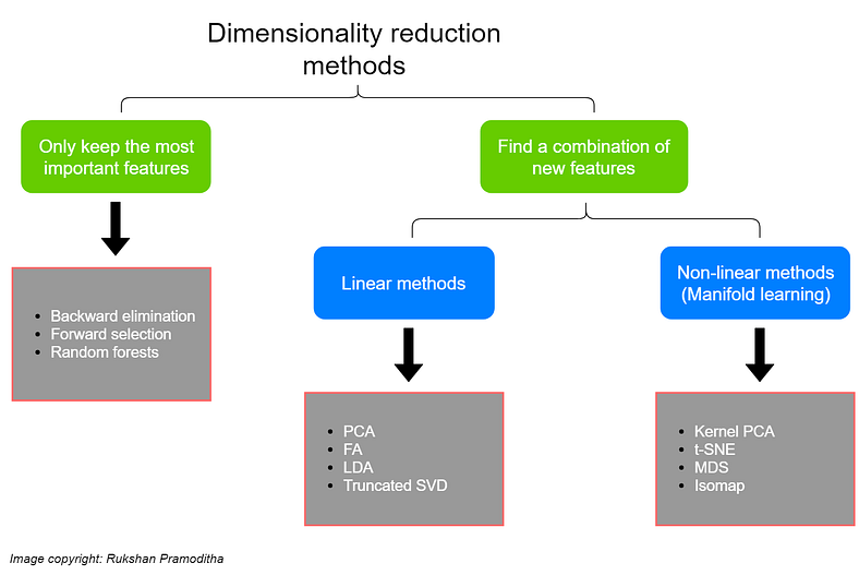
High Dimension Data Analysis - A tutorial and review for Dimensionality Reduction Techniques
This article explains and provides a comparative study of a few techniques for dimensionality reduction. It dives into the mathematical explanation of several feature selection and feature transformation techniques, while also providing the algorithmic representation and implementation of some other techniques. Lastly, it also provides a very brief review of various other works done in this space.
29 points
0 issues