Introduction to Bias-Variance and Error Analysis

1. The Bias-Variance Tradeoff
Assume you are given a well fitted machine learning model
You now realize that this MSE is too high, and try to find an explanation to this result:
-
Overfitting: the model is too closely related to the examples in the training set and doesn't generalize well to other examples.
-
Underfitting: the model didn't gather enough information from the training set, and doesn't capture the link between the features
and the target . -
The data is simply noisy, that is the model is neither overfitting or underfitting, and the high MSE is simply due to the amount of noise in the dataset.
Our intuition can be formalized by the Bias-Variance tradeoff.
Assume that the points in your training/test set are all taken from a similar distribution, with
and your goal is to compute
We can now compute our MSE on the test set by computing the following expectation with respect to the possible training sets (since
There is nothing we can do about the first term
To sum up, we can understand our MSE as follows
Hence, when analyzing the performance of a machine learning algorithm, we must always ask ourselves how to reduce the bias without increasing the variance, and respectively how to reduce the variance without increasing the bias. Most of the time, reducing one will increase the other, and there is a tradeoff between bias and variance.
2. Error Analysis
Even though understanding whether our poor test error is due to high bias or high variance is important, knowing which parts of the machine learning algorithm lead to this error or score is crucial.
Consider the machine learning pipeline on figure 1.
The algorithms is divided into several steps
-
The inputs are taken from a camera image
-
Preprocessing to remove the background on the image. For instance, if the image are taken from a security camera, the background is always the same, and we could remove it easily by keeping the pixels that changed on the image.
-
Detect the position of the face.
-
Detect the eyes - Detect the nose - Detect the mouth
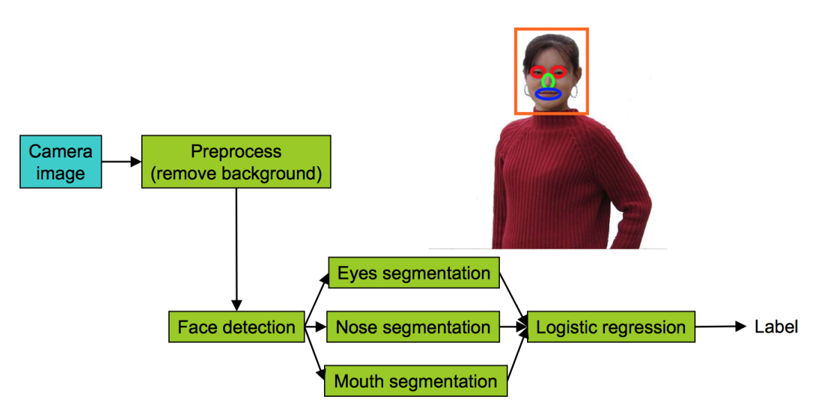
Figure 1: Face recognition pipeline
- Final logistic regression step to predict the label
If you biuld a complicated system like this one, you might want to figure out how much error is attributable to each of the components, how good is each of these green boxes. Indeed, if one of these boxes is really problematic, you might want to spend more time trying to improve the performance of that one green box. How do you decide what part to focus on?
One thing we can do is plug in the ground-truth for each component, and see how accuracy changes. Let's say the overall accuracy of the system is
Now let's say the accuracy only improves by
Now let's give the pipeline the perfect face detection by specifying the position of the face manually, see how much we improve the performance, and so on.
The results are specified in the table 1.
Looking at the table, we know that working on the background removal won't help much. It also tells us where the biggest jumps are. We notice that having an accurate face detection mechanism really improves the performance, and similarly, the eyes really help making the prediction more accurate.
Error analysis is also useful when publishing a paper, since it's a convenient way to
| Component | Accuracy |
| Overall system | |
| Preprocess (remove background) | |
| Face detection | |
| Eyes segmentation | |
| Nose segmentation | |
| Mouth segmentation | |
| Logistic regression |
Table 1: Accuracy when providing the system with the perfect component
analyze the error of an algorithm and explain which parts should be improved.
Ablative analysis
While error analysis tries to explain the difference between current performance and perfect performance, ablative analysis tries to explain the difference between some baseline (much poorer) performance and current performance.
For instance, suppose you have built a good anti-spam classifier by adding lots of clever features to logistic regression
-
Spelling correction
-
Sender host features
-
Email header features
-
Email text parser features
-
Javascript parser
-
Features from embedded images
and your question is: How much did each of these components really help?
In this example, let's say that simple logistic regression without any clever features gets
When presenting the results in a paper, ablative analysis really helps analyzing the features that helped decreasing the misclassification rate. Instead of simply giving the loss/error rate of the algorithm, we can provide evidence that some specific features are actually more important than others.
| Component | Accuracy |
| Overall system | |
| Spelling correction | |
| Sender host features | |
| Email header features | |
| Email text parser features | |
| Javascript parser | |
| Features from images |
Table 2: Accuracy when removing feature from logistic regression
Analyze your mistakes
Assume you are given a dataset with pictures of animals, and your goal is to identify pictures of cats that you would eventually send to the members of a community of cat lovers. You notice that there are many pictures of dogs in the original dataset, and wonders whether you should build a special algorithm to identify the pictures of dogs and avoid sending dogs pictures to cat lovers or not.
One thing you can do is take a
By analyzing your mistakes, you can focus on what's really important. If you notice that 80 out of your 100 mistakes are blurry images, then work hard on classifying correctly these blurry images. If you notice that 70 out of the 100 errors are great cats, then focus on this specific task of identifying great cats.
In brief, do not waste your time improving parts of your algorithm that won't really help decreasing your error rate, and focus on what really matters.
Recommended for you
A New Paradigm for Exploiting Pre-trained Model Hubs
A New Paradigm for Exploiting Pre-trained Model Hubs
It is often overlooked that the number of models in pre-trained model hubs is scaling up very fast. As a result, pre-trained model hubs are popular but under-exploited. Here a new paradigm is advocated to sufficiently exploit pre-trained model hubs.
