The Expectation Maximization Algorithm

You can read the notes from the previous lecture from Andrew Ng's CS229 course on the Mixtures of Gaussians and the EM algorithm here.

In the previous set of notes, we talked about the EM algorithm as applied to fitting a mixture of Gaussians. In this set of notes, we give a broader view of the EM algorithm, and show how it can be applied to a large family of estimation problems with latent variables. We begin our discussion with a very useful result called Jensen's inequality

1. Jensen's inequality

Let

f

be a function whose domain is the set of real numbers. Recall that

f

is a convex function if

f^{''} (x) \geq 0

(for all

x \in R

). In the case of

f

taking vector-valued inputs, this is generalized to the condition that its hessian

H

is positive semi-definite

(H \geq 0)

. If

f^{''} (x) > 0

for all

x

, then we say

f

is strictly convex (in the vector-valued case, the corresponding statement is that

H

must be positive definite, written

H > 0

). Jensen's inequality can then be stated as follows:

Theorem. Let

f

be a convex function, and let

X

be a random variable. Then:

E [f (X)] \geq f (E X) .

Moreover, if

f

is strictly convex, then

E [f (X)] = f (E X)

holds true if and only if

X = E [X]

with probability

1

(i.e., if

X

is a constant).

Recall our convention of occasionally dropping the parentheses when writing expectations, so in the theorem above,

f (E X) = f (E [X])

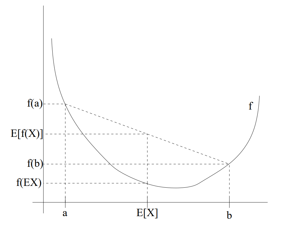
For an interpretation of the theorem, consider the figure below.

Here,

f

is a convex function shown by the solid line. Also,

X

is a random variable that has a

0.5

chance of taking the value

a

, and a

0.5

chance of taking the value

b

(indicated on the

x

-axis). Thus, the expected value of

X

is given by the midpoint between

a

and

b

We also see the values

f (a), f (b)

and

f (E [X])

indicated on the

y

-axis. Moreover, the value

E [f (X)]

is now the midpoint on the

y

-axis between

f (a)

and

f (b)

. From our example, we see that because

f

is convex, it must be the case that

E [f (X)] \geq f (E X)

Incidentally, quite a lot of people have trouble remembering which way the inequality goes, and remembering a picture like this is a good way to quickly figure out the answer.

Remark. Recall that

f

is [strictly] concave if and only if

- f

is [strictly] convex (i.e.,

f^{''} (x) \leq 0

H \leq 0

). Jensen's inequality also holds for concave functions

f

, but with the direction of all the inequalities reversed (

E [f (X)] \leq f (E X)

, etc.).

2. The EM algorithm

Suppose we have an estimation problem in which we have a training set

{x^{(1)}, \dots, x^{(n)}}

consisting of

n

independent examples. We have a latent variable model

p (x, z; θ)

with

z

being the latent variable (which for simplicity is assumed to take finite number of values). The density for

x

can be obtained by marginalized over the latent variable

z

\begin{matrix} (1) & p (x; θ) = \sum_{z} p (x, z; θ) \end{matrix}

We wish to fit the parameters

θ

by maximizing the log-likelihood of the data, defined by

\begin{matrix} (2) & ℓ (θ) = \sum_{i = 1}^{n} \log p (x^{(i)}; θ) \end{matrix}

We can rewrite the objective in terms of the joint density

p (x, z; θ)

\begin{aligned} (3) & ℓ (θ) & = \sum_{i = 1}^{n} \log p (x^{(i)}; θ) \\ (4) & = \sum_{i = 1}^{n} \log \sum_{z^{(i)}} p (x^{(i)}, z^{(i)}; θ) . \end{aligned}

But, explicitly finding the maximum likelihood estimates of the parameters

θ

may be hard since it will result in difficult non-convex optimization problems.^[1] Here, the

z^{(i)}

's are the latent random variables; and it is often the case that if the

z^{(i)}

's were observed, then maximum likelihood estimation would be easy.

In such a setting, the EM algorithm gives an efficient method for maximum likelihood estimation. Maximizing

ℓ (θ)

explicitly might be difficult, and our strategy will be to instead repeatedly construct a lower-bound on

ℓ

(E-step), and then optimize that lower-bound (M-step).^[2]

It turns out that the summation

\sum_{i = 1}^{n}

is not essential here, and towards a simpler exposition of the EM algorithm, we will first consider optimizing the the likelihood

\log p (x)

for a single example

x

. After we derive the algorithm for optimizing

\log p (x)

, we will convert it to an algorithm that works for

n

examples by adding back the sum to each of the relevant equations. Thus, now we aim to optimize

\log p (x; θ)

which can be rewritten as

\begin{matrix} (5) & \log p (x; θ) = \log \sum_{z} p (x, z; θ) \end{matrix}

Let

Q

be a distribution over the possible values of

z

. That is,

\sum_{z} Q (z) = 1

Q (z) \geq 0)

Consider the following:^[3]

\begin{aligned} \log p (x; θ) & = \log \sum_{z} p (x, z; θ) \\ (6) & = \log \sum_{z} Q (z) \frac{p (x, z; θ)}{Q (z)} \\ (7) & \geq \sum_{z} Q (z) \log \frac{p (x, z; θ)}{Q (z)} \end{aligned}

The last step of this derivation used Jensen's inequality. Specifically,

f (x) = \log x

is a concave function, since

f^{''} (x) = - 1 / x^{2} < 0

over its domain

x \in R^{+}

. Also, the term

\sum_{z} Q (z) [\frac{p (x, z; θ)}{Q (z)}]

in the summation is just an expectation of the quantity

[p (x, z; θ) / Q (z)]

with respect to

z

drawn according to the distribution given by

Q

.^[4] By Jensen's inequality, we have

f (E_{z \sim Q} [\frac{p (x, z; θ)}{Q (z)}]) \geq E_{z \sim Q} [f (\frac{p (x, z; θ)}{Q (z)})],

where the "

z \sim Q

" subscripts above indicate that the expectations are with respect to

z

drawn from

Q

. This allowed us to go from Equation (6) to Equation (7).

Now, for any distribution

Q

, the formula (7) gives a lower-bound on

\log p (x; θ)

. There are many possible choices for the

Q

's. Which should we choose? Well, if we have some current guess

θ

of the parameters, it seems natural to try to make the lower-bound tight at that value of

θ

. I.e., we will make the inequality above hold with equality at our particular value of

θ

To make the bound tight for a particular value of

θ

, we need for the step involving Jensen's inequality in our derivation above to hold with equality.

For this to be true, we know it is sufficient that the expectation be taken over a "constant"-valued random variable. I.e., we require that

\frac{p (x, z; θ)}{Q (z)} = c

for some constant

c

that does not depend on

z

. This is easily accomplished by choosing

Q (z) \propto p (x, z; θ) .

Actually, since we know

\sum_{z} Q (z) = 1

(because it is a distribution), this further tells us that

\begin{aligned} Q (z) & = \frac{p (x, z; θ)}{\sum_{z} p (x, z; θ)} \\ = \frac{p (x, z; θ)}{p (x; θ)} \\ (8) & = p (z | x; θ) \end{aligned}

Thus, we simply set the

Q

's to be the posterior distribution of the

z

's given

x

and the setting of the parameters

θ

Indeed, we can directly verify that when

Q (z) = p (z | x; θ)

, then equation (7) is an equality because

\begin{aligned} \sum_{z} Q (z) \log \frac{p (x, z; θ)}{Q (z)} & = \sum_{z} p (z | x; θ) \log \frac{p (x, z; θ)}{p (z | x; θ)} \\ = \sum_{z} p (z | x; θ) \log \frac{p (z | x; θ) p (x; θ)}{p (z | x; θ)} \\ = \sum_{z} p (z | x; θ) \log p (x; θ) \\ = \log p (x; θ) \sum_{z} p (z | x; θ) \\ = \log p (x; θ) (because \sum_{z} p (z | x; θ) = 1) \end{aligned}

For convenience, we call the expression in Equation (7) the evidence lower bound (ELBO) and we denote it by

\begin{matrix} (9) & ELBO (x; Q, θ) = \sum_{z} Q (z) \log \frac{p (x, z; θ)}{Q (z)} \end{matrix}

With this equation, we can re-write equation (7) as

\begin{matrix} (10) & \forall Q, θ, x, \log p (x; θ) \geq ELBO (x; Q, θ) \end{matrix}

Intuitively, the EM algorithm alternatively updates

Q

and

θ

by a) setting

Q (z) = p (z | x; θ)

following Equation (8) so that

ELBO (x; Q, θ) = \log p (x; θ)

for

x

and the current

θ

, and b) maximizing

ELBO (x; Q, θ)

w.r.t

θ

while fixing the choice of

Q

Recall that all the discussion above was under the assumption that we aim to optimize the log-likelihood

\log p (x; θ)

for a single example

x

. It turns out that with multiple training examples, the basic idea is the same and we only needs to take a sum over examples at relevant places. Next, we will build the evidence lower bound for multiple training examples and make the EM algorithm formal.

Recall we have a training set

{x^{(1)}, \dots, x^{(n)}}

. Note that the optimal choice of

Q

p (z | x; θ)

, and it depends on the particular example

x

. Therefore here we will introduce

n

distributions

Q_{1}, \dots, Q_{n}

, one for each example

x^{(i)}

. For each example

x^{(i)}

, we can build the evidence lower bound

\log p (x^{(i)}; θ) \geq ELBO (x^{(i)}; Q_{i}, θ) = \sum_{z^{(i)}} Q_{i} (z^{(i)}) \log \frac{p (x^{(i)}, z^{(i)}; θ)}{Q_{i} (z^{(i)})}

Taking sum over all the examples, we obtain a lower bound for the loglikelihood

\begin{aligned} (11) & ℓ (θ) & \geq \sum_{i} ELBO (x^{(i)}; Q_{i}, θ) \\ = \sum_{i} \sum_{z^{(i)}} Q_{i} (z^{(i)}) \log \frac{p (x^{(i)}, z^{(i)}; θ)}{Q_{i} (z^{(i)})} \end{aligned}

For any set of distributions

Q_{1}, \dots, Q_{n}

, the formula (11) gives a lowerbound on

ℓ (θ)

, and analogous to the argument around equation (8), the

Q_{i}

that attains equality satisfies

Q_{i} (z^{(i)}) = p (z^{(i)} | x^{(i)}; θ)

Thus, we simply set the

Q_{i}

's to be the posterior distribution of the

z^{(i)}

's given

x^{(i)}

with the current setting of the parameters

θ

Now, for this choice of the

Q_{i}

's, Equation (11) gives a lower-bound on the loglikelihood

ℓ

that we're trying to maximize. This is the E-step. In the M-step of the algorithm, we then maximize our formula in Equation (11) with respect to the parameters to obtain a new setting of the

θ

's. Repeatedly carrying out these two steps gives us the EM algorithm, which is as follows:

Repeat until convergence {

(E-step) For each

i

, set

Q_{i} (z^{(i)}) := p (z^{(i)} ∣ x^{(i)}; θ) .

(M-step) Set

\begin{aligned} θ & := \arg max_{θ} \sum_{i = 1}^{n} ELBO (x^{(i)}; Q_{i}, θ) \\ (12) & = \arg max_{θ} \sum_{i} \sum_{z^{(i)}} Q_{i} (z^{(i)}) \log \frac{p (x^{(i)}, z^{(i)}; θ)}{Q_{i} (z^{(i)})} . \end{aligned}

}

How do we know if this algorithm will converge? Well, suppose

θ^{(t)}

and

θ^{(t + 1)}

are the parameters from two successive iterations of EM. We will now prove that

ℓ (θ^{(t)}) \leq ℓ (θ^{(t + 1)})

, which shows EM always monotonically improves the log-likelihood. The key to showing this result lies in our choice of the

Q_{i}

's. Specifically, on the iteration of EM in which the parameters had started out as

θ^{(t)}

, we would have chosen

Q_{i}^{(t)} (z^{(i)}) := p (z^{(i)} | x^{(i)}; θ^{(t)})

. We saw earlier that this choice ensures that Jensen's inequality, as applied to get Equation (11), holds with equality, and hence

\begin{matrix} (13) & ℓ (θ^{(t)}) = \sum_{i = 1}^{n} ELBO (x^{(i)}; Q_{i}^{(t)}, θ^{(t)}) \end{matrix}

The parameters

θ^{(t + 1)}

are then obtained by maximizing the right hand side of the equation above. Thus,

\begin{aligned} ℓ (θ^{(t + 1)}) & \geq \sum_{i = 1}^{n} ELBO (x^{(i)}; Q_{i}^{(t)}, θ^{(t + 1)}) \\ (because inequality (11) holds for all Q and θ) \\ \geq \sum_{i = 1}^{n} ELBO (x^{(i)}; Q_{i}^{(t)}, θ^{(t)}) & (see reason below) \\ = ℓ (θ^{(t)}) & (by equation (13)) \end{aligned}

where the last inequality follows from that

θ^{(t + 1)}

is chosen explicitly to be

\arg max_{θ} \sum_{i = 1}^{n} ELBO (x^{(i)}; Q_{i}^{(t)}, θ)

Hence, EM causes the likelihood to converge monotonically. In our description of the EM algorithm, we said we'd run it until convergence. Given the result that we just showed, one reasonable convergence test would be to check if the increase in

ℓ (θ)

between successive iterations is smaller than some tolerance parameter, and to declare convergence if EM is improving

ℓ (θ)

too slowly.

Remark. If we define

(

by overloading

ELBO (\cdot))

\begin{matrix} (14) & ELBO (Q, θ) = \sum_{i = 1}^{n} ELBO (x^{(i)}; Q_{i}, θ) = \sum_{i} \sum_{z^{(i)}} Q_{i} (z^{(i)}) \log \frac{p (x^{(i)}, z^{(i)}; θ)}{Q_{i} (z^{(i)})} \end{matrix}

then we know

ℓ (θ) \geq ELBO (Q, θ)

from our previous derivation. The EM can also be viewed an alternating maximization algorithm on

ELBO (Q, θ)

, in which the E-step maximizes it with respect to

Q

(check this yourself), and the M-step maximizes it with respect to

θ

2.1. Other interpretation of ELBO

Let

ELBO (x; Q, θ) = \sum_{z} Q (z) \log \frac{p (x, z; θ)}{Q (z)}

be defined as in equation (9). There are several other forms of ELBO. First, we can rewrite

\begin{aligned} ELBO (x; Q, θ) & = E_{z \sim Q} [\log p (x, z; θ)] - E_{z \sim Q} [\log Q (z)] \\ (15) & = E_{z \sim Q} [\log p (x | z; θ)] - D_{K L} (Q ∥ p_{z}) \end{aligned}

where we use

p_{z}

to denote the marginal distribution of

z

(under the distribution

p (x, z; θ))

, and

D_{K L} ()

denotes the KL divergence

\begin{matrix} (16) & D_{K L} (Q ∥ p_{z}) = \sum_{z} Q (z) \log \frac{Q (z)}{p (z)} \end{matrix}

In many cases, the marginal distribution of

z

does not depend on the parameter

θ

. In this case, we can see that maximizing ELBO over

θ

is equivalent to maximizing the first term in (15). This corresponds to maximizing the conditional likelihood of

x

conditioned on

z

, which is often a simpler question than the original question.

Another form of

ELBO (\cdot)

is (please verify yourself)

\begin{matrix} (17) & ELBO (x; Q, θ) = \log p (x) - D_{K L} (Q ∥ p_{z | x}) \end{matrix}

where

p_{z | x}

is the conditional distribution of

z

given

x

under the parameter

θ

. This forms shows that the maximizer of

ELBO (Q, θ)

over

Q

is obtained when

Q = p_{z | x}

, which was shown in equation (8) before.

3. Mixture of Gaussians revisited

Armed with our general definition of the EM algorithm, let's go back to our old example of fitting the parameters

ϕ, μ

and

Σ

in a mixture of Gaussians. For the sake of brevity, we carry out the derivations for the M-step updates only for

ϕ

and

μ_{j}

, and leave the updates for

Σ_{j}

as an exercise for the reader.

The E-step is easy. Following our algorithm derivation above, we simply calculate

w_{j}^{(i)} = Q_{i} (z^{(i)} = j) = P (z^{(i)} = j | x^{(i)}; ϕ, μ, Σ) .

Here, "

Q_{i} (z^{(i)} = j)

" denotes the probability of

z^{(i)}

taking the value

j

under the distribution

Q_{i}

Next, in the M-step, we need to maximize, with respect to our parameters

ϕ, μ, Σ

, the quantity

\begin{aligned} \sum_{i = 1}^{n} & \sum_{z^{(i)}} Q_{i} (z^{(i)}) \log \frac{p (x^{(i)}, z^{(i)}; ϕ, μ, Σ)}{Q_{i} (z^{(i)})} \\ = \sum_{i = 1}^{n} \sum_{j = 1}^{k} Q_{i} (z^{(i)} = j) \log \frac{p (x^{(i)} ∣ z^{(i)} = j; μ, Σ) p (z^{(i)} = j; ϕ)}{Q_{i} (z^{(i)} = j)} \\ = \sum_{i = 1}^{n} \sum_{j = 1}^{k} w_{j}^{(i)} \log \frac{\frac{1}{(2 π)^{d / 2} {| Σ_{j} |}^{1 / 2}} \exp (- \frac{1}{2} {(x^{(i)} - μ_{j})}^{T} Σ_{j}^{- 1} (x^{(i)} - μ_{j})) \cdot ϕ_{j}}{w_{j}^{(i)}} \end{aligned}

Let's maximize this with respect to

μ_{l}

. If we take the derivative with respect to

μ_{l}

, we find

\begin{aligned} \nabla_{μ_{l}} & \sum_{i = 1}^{n} \sum_{j = 1}^{k} w_{j}^{(i)} \log \frac{\frac{1}{(2 π)^{d / 2} {| Σ_{j} |}^{1 / 2}} \exp (- \frac{1}{2} {(x^{(i)} - μ_{j})}^{T} Σ_{j}^{- 1} (x^{(i)} - μ_{j})) \cdot ϕ_{j}}{w_{j}^{(i)}} \\ = - \nabla_{μ_{l}} \sum_{i = 1}^{n} \sum_{j = 1}^{k} w_{j}^{(i)} \frac{1}{2} {(x^{(i)} - μ_{j})}^{T} Σ_{j}^{- 1} (x^{(i)} - μ_{j}) \\ = \frac{1}{2} \sum_{i = 1}^{n} w_{l}^{(i)} \nabla_{μ_{l}} 2 μ_{l}^{T} Σ_{l}^{- 1} x^{(i)} - μ_{l}^{T} Σ_{l}^{- 1} μ_{l} \\ = \sum_{i = 1}^{n} w_{l}^{(i)} (Σ_{l}^{- 1} x^{(i)} - Σ_{l}^{- 1} μ_{l}) \end{aligned}

Setting this to zero and solving for

μ_{l}

therefore yields the update rule

μ_{l} := \frac{\sum_{i = 1}^{n} w_{l}^{(i)} x^{(i)}}{\sum_{i = 1}^{n} w_{l}^{(i)}},

which was what we had in the previous set of notes.

Let's do one more example, and derive the M-step update for the parameters

ϕ_{j}

. Grouping together only the terms that depend on

ϕ_{j}

, we find that we need to maximize

\sum_{i = 1}^{n} \sum_{j = 1}^{k} w_{j}^{(i)} \log ϕ_{j} .

However, there is an additional constraint that the

ϕ_{j}

's sum to

1

, since they represent the probabilities

ϕ_{j} = p (z^{(i)} = j; ϕ)

. To deal with the constraint that

\sum_{j = 1}^{k} ϕ_{j} = 1

, we construct the Lagrangian

L (ϕ) = \sum_{i = 1}^{n} \sum_{j = 1}^{k} w_{j}^{(i)} \log ϕ_{j} + β (\sum_{j = 1}^{k} ϕ_{j} - 1),

where

β

is the Lagrange multiplier.^[5] Taking derivatives, we find

\frac{\partial}{\partial ϕ_{j}} L (ϕ) = \sum_{i = 1}^{n} \frac{w_{j}^{(i)}}{ϕ_{j}} + β

Setting this to zero and solving, we get

ϕ_{j} = \frac{\sum_{i = 1}^{n} w_{j}^{(i)}}{- β}

I.e.,

ϕ_{j} \propto \sum_{i = 1}^{n} w_{j}^{(i)}

. Using the constraint that

\sum_{j} ϕ_{j} = 1

, we easily find that

- β = \sum_{i = 1}^{n} \sum_{j = 1}^{k} w_{j}^{(i)} = \sum_{i = 1}^{n} 1 = n

. (This used the fact that

w_{j}^{(i)} = Q_{i} (z^{(i)} = j)

, and since probabilities sum to

1, \sum_{j} w_{j}^{(i)} = 1

.) We therefore have our M-step updates for the parameters

ϕ_{j}

ϕ_{j} := \frac{1}{n} \sum_{i = 1}^{n} w_{j}^{(i)} .

The derivation for the M-step updates to

Σ_{j}

are also entirely straightforward.

4. Variational inference and variational auto-encoder

Loosely speaking, variational auto-encoder [2] generally refers to a family of algorithms that extend the EM algorithms to more complex models parameterized by neural networks. It extends the technique of variational inference with the additional "re-parametrization trick" which will be introduced below. Variational auto-encoder may not give the best performance for many datasets, but it contains several central ideas about how to extend EM algorithms to high-dimensional continuous latent variables with non-linear models. Understanding it will likely give you the language and backgrounds to understand various recent papers related to it.

As a running example, we will consider the following parameterization of

p (x, z; θ)

by a neural network. Let

θ

be the collection of the weights of a neural network

g (z; θ)

that maps

z \in R^{k}

R^{d}

. Let

\begin{aligned} (18) & z & \sim N (0, I_{k \times k}) \\ (19) & x | z & \sim N (g (z; θ), σ^{2} I_{d \times d}) \end{aligned}

Here

I_{k \times k}

denotes identity matrix of dimension

k

k

, and

σ

is a scalar that we assume to be known for simplicity.

For the Gaussian mixture models in Section 3, the optimal choice of

Q (z) = p (z | x; θ)

for each fixed

θ

, that is the posterior distribution of

z

, can be analytically computed. In many more complex models such as the model (19), it's intractable to compute the exact the posterior distribution

p (z | x; θ)

Recall that from equation (10), ELBO is always a lower bound for any choice of

Q

, and therefore, we can also aim for finding an approximation of the true posterior distribution. Often, one has to use some particular form to approximate the true posterior distribution. Let

Q

be a family of

Q

's that we are considering, and we will aim to find a

Q

within the family of

Q

that is closest to the true posterior distribution. To formalize, recall the definition of the ELBO lower bound as a function of

Q

and

θ

defined in equation (14)

ELBO (Q, θ) = \sum_{i = 1}^{n} ELBO (x^{(i)}; Q_{i}, θ) = \sum_{i} \sum_{z^{(i)}} Q_{i} (z^{(i)}) \log \frac{p (x^{(i)}, z^{(i)}; θ)}{Q_{i} (z^{(i)})}

Recall that EM can be viewed as alternating maximization of

ELBO (Q, θ)

. Here instead, we optimize the EBLO over

Q \in Q

\begin{matrix} (20) & max_{Q \in Q} max_{θ} ELBO (Q, θ) \end{matrix}

Now the next question is what form of

Q

(or what structural assumptions to make about

Q

) allows us to efficiently maximize the objective above. When the latent variable

z

are high-dimensional discrete variables, one popular assumption is the mean field assumption, which assumes that

Q_{i} (z)

gives a distribution with independent coordinates, or in other words,

Q_{i}

can be decomposed into

Q_{i} (z) = Q_{i}^{1} (z_{1}) \dots Q_{i}^{k} (z_{k})

. There are tremendous applications of mean field assumptions to learning generative models with discrete latent variables, and we refer to [1] for a survey of these models and their impact to a wide range of applications including computational biology, computational neuroscience, social sciences. We will not get into the details about the discrete latent variable cases, and our main focus is to deal with continuous latent variables, which requires not only mean field assumptions, but additional techniques.

When

z \in R^{k}

is a continuous latent variable, there are several decisions to make towards successfully optimizing (20). First we need to give a succinct representation of the distribution

Q_{i}

because it is over an infinite number of points. A natural choice is to assume

Q_{i}

is a Gaussian distribution with some mean and variance. We would also like to have more succinct representation of the means of

Q_{i}

of all the examples. Note that

Q_{i} (z^{(i)})

is supposed to approximate

p (z^{(i)} | x^{(i)}; θ)

. It would make sense let all the means of the

Q_{i}

's be some function of

x^{(i)}

. Concretely, let

q (\cdot; ϕ), v (\cdot; ϕ)

be two functions that map from dimension

d

k

, which are parameterized by

ϕ

and

ψ

, we assume that

\begin{matrix} (21) & Q_{i} = N (q (x^{(i)}; ϕ), diag {(v (x^{(i)}; ψ))}^{2}) \end{matrix}

Here

diag (w)

means the

k \times k

matrix with the entries of

w \in R^{k}

on the diagonal. In other words, the distribution

Q_{i}

is assumed to be a Gaussian distribution with independent coordinates, and the mean and standard deviations are governed by

q

and

v

. Often in variational auto-encoder,

q

and

v

are chosen to be neural networks.^[6] In recent deep learning literature, often

q, v

are called encoder (in the sense of encoding the data into latent code), whereas

g (z; θ)

if often referred to as the decoder.

We remark that

Q_{i}

of such form in many cases are very far from a good approximation of the true posterior distribution. However, some approximation is necessary for feasible optimization. In fact, the form of

Q_{i}

needs to satisfy other requirements (which happened to be satisfied by the form (21))

Before optimizing the ELBO, let's first verify whether we can efficiently evaluate the value of the ELBO for fixed

Q

of the form (21) and

θ

. We rewrite the ELBO as a function of

ϕ, ψ, θ

\begin{aligned} (22) & ELBO (ϕ, ψ, θ) & = \sum_{i = 1}^{n} E_{z^{(i)} \sim Q_{i}} [\log \frac{p (x^{(i)}, z^{(i)}; θ)}{Q_{i} (z^{(i)})}] \\ where Q_{i} = N (q (x^{(i)}; ϕ), diag (v (x^{(i)}; ψ))^{2}) \end{aligned}

Note that to evaluate

Q_{i} (z^{(i)})

inside the expectation, we should be able to compute the density of

Q_{i}

. To estimate the expectation

E_{z^{(i)} \sim Q_{i}}

, we should be able to sample from distribution

Q_{i}

so that we can build an empirical estimator with samples. It happens that for Gaussian distribution

Q_{i} = N (q (x^{(i)}; ϕ), diag (v (x^{(i)}; ψ))^{2})

, we are able to be both efficiently.

Now let's optimize the ELBO. It turns out that we can run gradient ascent over

ϕ, ψ, θ

instead of alternating maximization. There is no strong need to compute the maximum over each variable at a much greater cost. (For Gaussian mixture model in Section 3, computing the maximum is analytically feasible and relatively cheap, and therefore we did alternating maximization.) Mathematically, let

η

be the learning rate, the gradient ascent step is

\begin{aligned} θ & := θ + η \nabla_{θ} ELBO (ϕ, ψ, θ) \\ ϕ & := ϕ + η \nabla_{ϕ} ELBO (ϕ, ψ, θ) \\ ψ & := ψ + η \nabla_{ψ} ELBO (ϕ, ψ, θ) \end{aligned}

Computing the gradient over

θ

is simple because

\begin{aligned} \nabla_{θ} ELBO (ϕ, ψ, θ) & = \nabla_{θ} \sum_{i = 1}^{n} E_{z^{(i)} \sim Q_{i}} [\frac{\log p (x^{(i)}, z^{(i)}; θ)}{Q_{i} (z^{(i)})}] \\ = \nabla_{θ} \sum_{i = 1}^{n} E_{z^{(i)} \sim Q_{i}} [\log p (x^{(i)}, z^{(i)}; θ)] \\ (23) & = \sum_{i = 1}^{n} E_{z^{(i)} \sim Q_{i}} [\nabla_{θ} \log p (x^{(i)}, z^{(i)}; θ)] \end{aligned}

But computing the gradient over

ϕ

and

ψ

is tricky because the sampling distribution

Q_{i}

depends on

ϕ

and

ψ

. (Abstractly speaking, the issue we face can be simplified as the problem of computing the gradient

E_{z \sim Q_{ϕ}} [f (ϕ)]

with respect to variable

ϕ

. We know that in general,

\nabla E_{z \sim Q_{ϕ}} [f (ϕ)] \neq

E_{z \sim Q_{ϕ}} [\nabla f (ϕ)]

because the dependency of

Q_{ϕ}

ϕ

has to be taken into account as well.)

The idea that comes to rescue is the so-called re-parameterization trick: we rewrite

z^{(i)} \sim Q_{i} = N (q (x^{(i)}; ϕ), diag {(v (x^{(i)}; ψ))}^{2})

in an equivalent way:

\begin{matrix} (24) & z^{(i)} = q (x^{(i)}; ϕ) + v (x^{(i)}; ψ) ⊙ ξ^{(i)} where ξ^{(i)} \sim N (0, I_{k \times k}) \end{matrix}

Here

x ⊙ y

denotes the entry-wise product of two vectors of the same dimension. Here we used the fact that

x \sim N (μ, σ^{2})

is equivalent to that

x = μ + ξ σ

with

ξ \sim N (0, 1)

. We mostly just used this fact in every dimension simultaneously for the random variable

z^{(i)} \sim Q_{i}

With this re-parameterization, we have that

\begin{aligned} (25) & E_{z^{(i)} \sim Q_{i}} [\log \frac{p (x^{(i)}, z^{(i)}; θ)}{Q_{i} (z^{(i)})}] \\ = E_{ξ^{(i)} \sim N (0, 1)} [\log \frac{p (x^{(i)}, q (x^{(i)}; ϕ) + v (x^{(i)}; ψ) ⊙ ξ^{(i)}; θ)}{Q_{i} (q (x^{(i)}; ϕ) + v (x^{(i)}; ψ) ⊙ ξ^{(i)})}] \end{aligned}

It follows that

\begin{aligned} \nabla_{ϕ} E_{z^{(i)} \sim Q_{i}} [\log \frac{p (x^{(i)}, z^{(i)}; θ)}{Q_{i} (z^{(i)})}] \\ = \nabla_{ϕ} E_{ξ^{(i)} \sim N (0, 1)} [\log \frac{p (x^{(i)}, q (x^{(i)}; ϕ) + v (x^{(i)}; ψ) ⊙ ξ^{(i)}; θ)}{Q_{i} (q (x^{(i)}; ϕ) + v (x^{(i)}; ψ) ⊙ ξ^{(i)})}] \\ = E_{ξ^{(i)} \sim N (0, 1)} [\nabla_{ϕ} \log \frac{p (x^{(i)}, q (x^{(i)}; ϕ) + v (x^{(i)}; ψ) ⊙ ξ^{(i)}; θ)}{Q_{i} (q (x^{(i)}; ϕ) + v (x^{(i)}; ψ) ⊙ ξ^{(i)})}] \end{aligned}

We can now sample multiple copies of

ξ^{(i)}

's to estimate the the expectation in the RHS of the equation above.^[7] We can estimate the gradient with respect to

ψ

similarly, and with these, we can implement the gradient ascent algorithm to optimize the ELBO over

ϕ, ψ, θ

There are not many high-dimensional distributions with analytically computable density function are known to be re-parameterizable. We refer to [2] for a few other choices that can replace Gaussian distribution.

You can read the notes from the next lecture from Andrew Ng's CS229 course on Factor Analysis here.

References

[1] David M Blei, Alp Kucukelbir, and Jon D McAuliffe. Variational inference: A review for statisticians. Journal of the American Statistical Association, 112(518):859-877, 2017 .

[2] Diederik P Kingma and Max Welling. Auto-encoding variational bayes. arXiv preprint arXiv:1312.6114, 2013.

It's mostly an empirical observation that the optimization problem is difficult to optimize. ↩︎
Empirically, the E-step and M-step can often be computed more efficiently than optimizing the function $ℓ (\cdot)$ directly. However, it doesn't necessarily mean that alternating the two steps can always converge to the global optimum of $ℓ (\cdot)$ . Even for mixture of Gaussians, the EM algorithm can either converge to a global optimum or get stuck, depending on the properties of the training data. Empirically, for real-world data, often EM can converge to a solution with relatively high likelihood (if not the optimum), and the theory behind it is still largely not understood. ↩︎
If $z$ were continuous, then $Q$ would be a density, and the summations over $z$ in our discussion are replaced with integrals over $z$ . ↩︎
We note that the notion $\frac{p (x, z; θ)}{Q (z)}$ only makes sense if $Q (z) \neq 0$ whenever $p (x, z; θ) \neq 0$ . Here we implicitly assume that we only consider those $Q$ with such a property. ↩︎
We don't need to worry about the constraint that $ϕ_{j} \geq 0$ , because as we'll shortly see, the solution we'll find from this derivation will automatically satisfy that anyway. ↩︎
$q$ and $v$ can also share parameters. We sweep this level of details under the rug in this note. ↩︎
Empirically people sometimes just use one sample to estimate it for maximum computational efficiency. ↩︎

The Expectation Maximization Algorithm

1. Jensen's inequality

2. The EM algorithm

2.1. Other interpretation of ELBO

3. Mixture of Gaussians revisited

4. Variational inference and variational auto-encoder

References

Recommended for you

Report Article