Mathematical model of bearing lubrication under themal conditions

Abstract

Most operations of machines operate under fluid film lubrication known as Elastohydrodynamic lubrication (EHL). Thermal behaviour is also an important aspect since most machines operate under heavy loads, high speeds and rough surfaces. Previous Thermal Elastohydrodynamic lubrication (TEHL) research has focused on Newtonian lubricants under full-film lubrication. The present study will develop a realistic model for non-Newtonian point contact of sliding/ rolling bearing capable of mathematical simulation of the lubrication regime. The mathematical model consists of the Reynolds-Eyring equation, film thickness equation, density and viscosity equations for rheology of lubricant which depend on pressure and temperature, and the energy equation for lubricant film.The equations are descritised using the finite different method and simulated by Matlab. Pressure and temperature profiles are also presented.

1. Introduction

In the history of lubrication there is great effort to understand the effect of temperature variation on Non-Newtonian lubricants. It is well known that rolling/ sliding bearings are often used under heavy load conditions and high speed [1]. Under the these conditions, any temperature increase can result to increase in friction and failures in the surface such as deformation, scuffing and sliding wear. Thus, thermal effects play an important factor for reliable simulation of machine components working under Elastohydrodynamic lubrication. Thermal effects at contact region causes frictional heat and may lead to failure of the bearing. The study of thermal effects has attracted many attention and challenge in research. Thus thermal effects play an important role and are significant in EHL study [2,3]. Experimental research in TEHL are still very difficult thus numerical simulations come in-handy in TEHL research. Greenwood et. al. [4] investigated thermal effects and concluded that the film thickness reduces at high velocities. ten Napel et al.[5] in their research showed that pressure was affected by temperature.Thus,thermal effects cannot be ignored in EHL. Thermal effects in EHL are usually modelled by interoperating the energy equation which is solved together with the Reynolds equation [6].\ Research in TEHL has mostly assumed Newtonian lubricants. It is a fact that no lubricants are Newtonian but Non-Newtonian. To better develop and predict TEHL simulation, Non-Newtonian lubricant has to be considered in this research. Many researchers have proposed various rheology models to in cooperate Non-Newtonian nature of lubricants [7]. In our research the Reynolds-Eyring model has been used since it is recommended by many researchers [8,9,10,11] for lubrication performance studies. Srikanth et. al [12] in their research used the finite difference method to solve to descritise the Reynold and energy equation. Kiogora et al. [13,14] were also able to solve the Reynold and Energy equations using the finite difference method which verified pressure and temperature values for pad thrust bearing\

2. Mathematical model

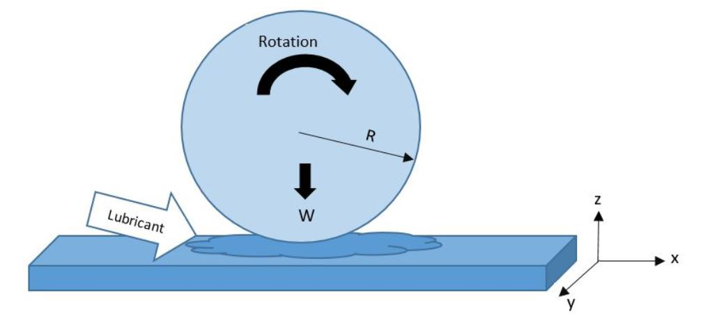
The mechanisms of TEHL that occur between the rolling elements and surface are described the geometry in figure 1
original image

2.1. Non-Newtonian Model

When two surfaces slide against each other, there is friction force that is generated by the two surfaces in contact. This friction in lubricants is referred to as viscosity. The Eyring model incorporates the Non-Newtonian nature of the lubricant so that the pressure dependence nature and the shear thinning of the fluid's viscosity [15] can be given by
(1) γ = τ η s i n h ( τ τ 0 ) (1) γ = τ η s i n h ( τ τ 0 ) {:(1)gamma=(tau )/(eta)sinh((tau)/(tau_(0))):}\begin{equation} \gamma=\frac{\tau}{\eta}sinh(\frac{\tau}{\tau_{0}}) \end{equation}

2.2. Reynold-Eyring Equation

The pressure between the two contact regions is described by the Reynold-Eyring equation for non-Newtonian lubricants for point contact.
(2) x [ ρ h 3 12 η p x S ( x ) ) ] + y [ ρ h 3 12 η p y Q ( y ) ) ] = U m 2 x ( ρ h ) + V m 2 y ( ρ h ) + t ( ρ h ) (2) x [ ρ h 3 12 η p x S ( x ) ) ] + y [ ρ h 3 12 η p y Q ( y ) ) ] = U m 2 x ( ρ h ) + V m 2 y ( ρ h ) + t ( ρ h ) {:(2)(del)/(del x)[(rhoh^(3))/(12 eta)(del p)/(del x)S(x))]+(del)/(del y)[(rhoh^(3))/(12 eta)(del p)/(del y)Q(y))]=(U_(m))/(2)(del)/(del x)(rho h)+(V_(m))/(2)(del)/(del y)(rho h)+(del)/(del t)(rho h):}\begin{equation} \frac{\partial}{\partial x} [\frac{\rho h^3}{12\eta}\frac{\partial p}{\partial x}S(x))] +\frac{\partial}{\partial y} [\frac{\rho h^3}{12\eta}\frac{\partial p}{\partial y}Q(y))]=\frac{U_m}{2}\frac{\partial}{\partial x}(\rho h)+\frac{V_m}{2}\frac{\partial}{\partial y}(\rho h)+\frac{\partial}{\partial t}(\rho h) \end{equation}
where
S ( x ) = 3 ( ϵ c o s h ( ϵ ) s i n h ( ϵ ) ) ϵ 3 c o s h ( τ m τ 0 ) S ( x ) = 3 ( ϵ c o s h ( ϵ ) s i n h ( ϵ ) ) ϵ 3 c o s h ( τ m τ 0 ) S(x)=(3(epsilon cosh(epsilon)-sinh(epsilon)))/(epsilon^(3))cosh((tau _(m))/(tau_(0)))S(x)=\frac{3(\epsilon cosh(\epsilon)-sinh(\epsilon))}{\epsilon^3}cosh(\frac{\tau_m}{\tau_0}) \hspace{1cm}
Q ( y ) = 3 ( δ c o s h ( δ ) s i n h ( δ ) ) δ 3 c o s h ( τ m τ 0 ) Q ( y ) = 3 ( δ c o s h ( δ ) s i n h ( δ ) ) δ 3 c o s h ( τ m τ 0 ) Q(y)=(3(delta cosh(delta)-sinh(delta)))/(delta^(3))cosh((tau _(m))/(tau_(0)))Q(y)=\frac{3(\delta cosh(\delta)-sinh(\delta))}{\delta^3}cosh(\frac{\tau_m}{\tau_0})

2.3. Film thickness Equation

The film thickness equation for point contact with surface roughness
(3) h ( x , y ) = h 00 + x 2 2 R + y 2 2 R + r r ( x , y ) + 2 π E p ( x , y ) ( x x ) 2 + ( y y ) 2 d x d y (3) h ( x , y ) = h 00 + x 2 2 R + y 2 2 R + r r ( x , y ) + 2 π E p ( x , y ) ( x x ) 2 + ( y y ) 2 d x d y {:(3)h(x","y)=h_(00)+(x^(2))/(2R)+(y^(2))/(2R)+rr(x","y)+(2)/(piE^('))int_(-oo)^(oo)int_(-oo)^(oo)(p(x^('),y^(')))/(sqrt((x-x^('))^(2)+(y-y^('))^(2)))dx^(')dy^('):}\begin{equation} h(x,y)=h_{00}+\frac{x^{2}}{2R}+\frac{y^{2}}{2R}+rr(x,y)+\frac{2}{\pi E'}\intop_{-\infty}^{\infty}\intop_{-\infty}^{\infty}\frac{p(x^{\prime},y^{\prime})}{\sqrt{(x-x^{\prime})^{2}+(y-y^{\prime})^{2}}}dx'dy^{\prime} \end{equation}

2.4. Viscosity Equation

The lubricant viscosity is assumed to be dependent on pressure and temperature hence we consider the Roeland"s model [16].
(4) η = η 0 exp [ l n ( η 0 ) + 9.67 ( 1 + ( 1 + 5.1 10 9 p ) Z ) ( θ 138 θ 0 138 ) S ] (4) η = η 0 exp [ l n ( η 0 ) + 9.67 ( 1 + ( 1 + 5.1 10 9 p ) Z ) ( θ 138 θ 0 138 ) S ] {:(4)eta=eta_(0)exp[ln(eta_(0))+9.67(-1+(1+5.1**10^(-)9p)^(Z))((theta-138)/(theta_(0)-138))^(-S)]:}\begin{equation} \eta=\eta_0 \exp[ln(\eta_0)+9.67(-1+(1+5.1*10^-9p)^Z)(\frac{\theta-138}{\theta_0 -138})^{-S}] \end{equation}

2.5. Density Equation

The compressibility of the lubricant has to be accounted for because of the high pressures due to elastohydrodynamic lubrication situations.The density equation proposed by Downson and Higginsin [17] is considered also to be a function of pressure and temperature
(5) ρ = ρ 0 [ 1 + 0.6 10 9 p 1 + 1.7 10 9 p 0.00065 ( θ θ 0 ) ] (5) ρ = ρ 0 [ 1 + 0.6 10 9 p 1 + 1.7 10 9 p 0.00065 ( θ θ 0 ) ] {:(5)rho=rho_(0)[1+(0.6**10^(-)9p)/(1+1.7**10^(-)9p)-0.00065(theta-theta_(0))]:}\begin{equation} \rho=\rho_0[1+\frac{0.6*10^-9p}{1+1.7*10^-9p}-0.00065(\theta-\theta_0)] \end{equation}

2.6. Non Dimensionalization

The equations are non-dimensionalized using the Hertzian dry contact variables below [18] .
ρ ¯ = ρ ρ 0 , η ¯ = η η 0 , X = x a , Y = y a ρ ¯ = ρ ρ 0 , η ¯ = η η 0 , X = x a , Y = y a bar(rho)=(rho)/(rho_(0)), bar(eta)=(eta)/(eta_(0)),X=(x)/(a),Y=(y)/(a)\bar{\rho}=\frac{\rho}{\rho_{0}},\bar{\eta}=\frac{\eta}{\eta_{0}},X=\frac{x}{a},Y=\frac{y}{a}
P = p p h , H = h R a 2 , T = t U m 2 a P = p p h , H = h R a 2 , T = t U m 2 a P=(p)/(p_(h)),H=(hR)/(a^(2)),T=(tU_(m))/(2a)P=\frac{p}{p_{h}},H=\frac{hR}{a^{2}},T=\frac{tU_{m}}{2a}
H 00 = h 00 R a 2 , θ ¯ = θ θ 0 , U = u η 0 R E , V = v η 0 R E H 00 = h 00 R a 2 , θ ¯ = θ θ 0 , U = u η 0 R E , V = v η 0 R E H_(00)=(h_(00)R)/(a^(2)), bar(theta)=(theta)/(theta_(0)),U=(ueta_(0))/(RE^(^('))),V=(veta_(0))/(RE^(^(')))H_{00}=\frac{h_{00}R}{a^{2}},\overline{\theta}=\frac{\theta}{\theta_{0}},U=\frac{u\eta_{0}}{RE^{'}},V=\frac{v\eta_{0}}{RE^{'}}
Dimensionless Reynold-Eyring Equation Applying the above non-dimensionless variables to the Reynold-Eyring equation becomes and assuming the rolling speed U m = V m U m = V m U_(m)=V_(m)U_{m}=V_{m} in the x and y direction is the same we have,
(6) X [ ρ ¯ H 3 η ¯ P X S ( x ) ] + Y [ ρ ¯ H 3 η ¯ P Y Q ( y ) ] = λ { X [ ρ ¯ H ] + Y [ ρ ¯ H ] + T [ ρ ¯ H ] } (6) X ρ ¯ H 3 η ¯ P X S ( x ) + Y ρ ¯ H 3 η ¯ P Y Q ( y ) = λ X ρ ¯ H + Y ρ ¯ H + T ρ ¯ H {:(6)(del)/(del X)[(( bar(rho))H^(3))/(( bar(eta)))(del P)/(del X)S(x)]+(del)/(del Y)[(( bar(rho))H^(3))/(( bar(eta)))(del P)/(del Y)Q(y)]=lambda{(del)/(del X)[( bar(rho))H]+(del)/(del Y)[( bar(rho))H]+(del)/(del T)[( bar(rho))H]}:}\begin{equation} \frac{\partial}{\partial X}\left[\frac{\bar{\rho}H^{3}}{\bar{\eta}}\frac{\partial P}{\partial X}S(x)\right]+\frac{\partial}{\partial Y}\left[\frac{\bar{\rho}H^{3}}{\bar{\eta}}\frac{\partial P}{\partial Y}Q(y)\right]=\lambda\left\{ \frac{\partial}{\partial X}\left[\bar{\rho}H\right]+\frac{\partial}{\partial Y}\left[\bar{\rho}H\right]+\frac{\partial}{\partial T}\left[\bar{\rho}H\right]\right\} \end{equation}
with
(7) S ( x ) = 3 ( ξ c o s h ( ξ ) s i n h ( ξ ) ) ξ 3 × 1 + [ R n 0 η ¯ ( U 2 U 1 ) τ 0 H a 2 ξ s i n ( ξ ) ] 2 (7) S ( x ) = 3 ξ c o s h ξ s i n h ξ ξ 3 × 1 + R n 0 η ¯ U 2 U 1 τ 0 H a 2 ξ s i n ξ 2 {:(7)S(x)=(3(xi cosh(xi)-sinh(xi)))/(xi^(3))xxsqrt(1+[(Rn_(0) bar(eta)(U_(2)-U_(1)))/(tau_(0)Ha^(2))(xi)/(sin(xi))]^(2)):}\begin{equation} S(x)=\frac{3\left(\xi cosh\left(\xi\right)-sinh\left(\xi\right)\right)}{\xi^{3}}\times\sqrt{1+\left[\frac{Rn_{0}\overline{\eta}\left(U_{2}-U_{1}\right)}{\tau_{0}Ha^{2}}\frac{\xi}{sin\left(\xi\right)}\right]^{2}} \end{equation}
(8) Q ( y ) = 3 ( δ c o s h ( δ ) s i n h ( δ ) ) δ 3 × 1 + [ R n 0 η ¯ ( V 2 V 1 ) τ 0 H a 2 δ s i n ( δ ) ] 2 (8) Q ( y ) = 3 δ c o s h δ s i n h δ δ 3 × 1 + R n 0 η ¯ V 2 V 1 τ 0 H a 2 δ s i n δ 2 {:(8)Q(y)=(3(delta cosh(delta)-sinh(delta)))/(delta^(3))xxsqrt(1+[(Rn_(0) bar(eta)(V_(2)-V_(1)))/(tau_(0)Ha^(2))(delta)/(sin(delta))]^(2)):}\begin{equation} Q(y)=\frac{3\left(\delta cosh\left(\delta\right)-sinh\left(\delta\right)\right)}{\delta^{3}}\times\sqrt{1+\left[\frac{Rn_{0}\overline{\eta}\left(V_{2}-V_{1}\right)}{\tau_{0}Ha^{2}}\frac{\delta}{sin\left(\delta\right)}\right]^{2}} \end{equation}
(9) λ = 6 η 0 U m R 2 p h a 3 , ξ = H a p h 2 R τ 0 P X δ = H a p h 2 R τ 0 P Y (9) λ = 6 η 0 U m R 2 p h a 3 , ξ = H a p h 2 R τ 0 P X δ = H a p h 2 R τ 0 P Y {:(9)lambda=(6eta_(0)U_(m)R^(2))/(p_(h)a^(3))","xi=(Hap_(h))/(2Rtau_(0))(del P)/(del X)delta=(Hap_(h))/(2Rtau_(0))(del P)/(del Y):}\begin{equation} \lambda=\frac{6\eta_{0}U_{m}R^{2}}{p_{h}a^{3}},\xi=\frac{Hap_{h}}{2R\tau_{0}}\frac{\partial P}{\partial X}\delta=\frac{Hap_{h}}{2R\tau_{0}}\frac{\partial P}{\partial Y} \end{equation}
if we let β = ρ ¯ H 3 η ¯ β = ρ ¯ H 3 η ¯ beta=(( bar(rho))H^(3))/(( bar(eta)))\beta=\frac{\bar{\rho}H^{3}}{\bar{\eta}},equation above becomes
(10) X [ β P X S ( x ) ] + Y [ β P Y Q ( y ) ] = λ { X [ ρ ¯ H ] + Y [ ρ ¯ H ] + T [ ρ ¯ H ] } (10) X β P X S ( x ) + Y β P Y Q ( y ) = λ X ρ ¯ H + Y ρ ¯ H + T ρ ¯ H {:(10)(del)/(del X)[beta(del P)/(del X)S(x)]+(del)/(del Y)[beta(del P)/(del Y)Q(y)]=lambda{(del)/(del X)[( bar(rho))H]+(del)/(del Y)[( bar(rho))H]+(del)/(del T)[( bar(rho))H]}:}\begin{equation} \frac{\partial}{\partial X}\left[\beta\frac{\partial P}{\partial X}S(x)\right]+\frac{\partial}{\partial Y}\left[\beta\frac{\partial P}{\partial Y}Q(y)\right]=\lambda\left\{ \frac{\partial}{\partial X}\left[\bar{\rho}H\right]+\frac{\partial}{\partial Y}\left[\bar{\rho}H\right]+\frac{\partial}{\partial T}\left[\bar{\rho}H\right]\right\} \end{equation}
Dimensionless Film Thickness Equation
(11) H ( X , Y ) = H 00 + X 2 2 + Y 2 2 + R R ( X , Y ) 2 π 2 P ( X , Y ) ( ( X X ) ) 2 + ( ( Y Y ) ) 2 d X d Y (11) H ( X , Y ) = H 00 + X 2 2 + Y 2 2 + R R ( X , Y ) 2 π 2 P ( X , Y ) ( ( X X ) ) 2 + ( ( Y Y ) ) 2 d X d Y {:(11)H(X","Y)=H_(00)+(X^(2))/(2)+(Y^(2))/(2)+RR(X","Y)(2)/(pi^(2))int_(-oo)^(oo)int_(-oo)^(oo)(P(X^('),Y^(')))/(sqrt(((X-X^(')))^(2)+((Y-Y^(')))^(2)))dX^(')dY^(^(')):}\begin{equation} H(X,Y)=H_{00}+\frac{X^{2}}{2}+\frac{Y^{2}}{2}+RR(X,Y)\frac{2}{\pi^{2}}\intop_{-\infty}^{\infty}\intop_{-\infty}^{\infty}\frac{P(X^{\prime},Y^{\prime})}{\sqrt{((X-X^{\prime}))^{2}+((Y-Y^{\prime}))^{2}}}dX'dY^{'} \end{equation}
Dimensionless Lubricant viscosity equation
(12) η ¯ = e x p [ l n ( η 0 ) + 9.67 × [ 1 + ( 1 + 5.1 10 9 P p h ) Z ] ( θ ¯ θ 0 138 θ 0 138 ) S ] (12) η ¯ = e x p [ l n ( η 0 ) + 9.67 × [ 1 + ( 1 + 5.1 10 9 P p h ) Z ] ( θ ¯ θ 0 138 θ 0 138 ) S ] {:(12) bar(eta)=exp[ln(eta_(0))+9.67 xx[-1+(1+5.1**10^(-9)Pp_(h))^(Z)](( bar(theta)theta_(0)-138)/(theta_(0)-138))^(-S)]:}\begin{equation} \overline{\eta}=exp[ln(\eta_{0})+9.67\times[-1+(1+5.1*10^{-9}Pp_{h})^{Z}](\frac{\overline{\theta}\theta_{0}-138}{\theta_{0}-138})^{-S}] \end{equation}
Dimensionless Lubricants Density Equation
(13) ρ ¯ = [ 1 + 0.6 10 9 P p h 1 + 1.7 10 9 P p h 0.00065 θ 0 ( θ ¯ 1 ) ] (13) ρ ¯ = 1 + 0.6 10 9 P p h 1 + 1.7 10 9 P p h 0.00065 θ 0 θ ¯ 1 {:(13) bar(rho)=[1+(0.6**10^(-9)Pp_(h))/(1+1.7**10^(-9)Pp_(h))-0.00065theta_(0)( bar(theta)-1)]:}\begin{equation} \overline{\rho}=\left[1+\frac{0.6*10^{-9}Pp_{h}}{1+1.7*10^{-9}Pp_{h}}-0.00065\theta_{0}\left(\overline{\theta}-1\right)\right] \end{equation}

2.7. Boundary Conditions

The TEHL equations are discretised on a rectangular domain X i n X X e n d X i n X X e n d X_(in) <= X <= X_(end)X_{in}\leq X\leq X_{end} and Y i n Y Y e n d Y i n Y Y e n d Y_(in) <= Y <= Y_(end)Y_{in}\leq Y\leq Y_{end}.Thus the boundary conditions are,
P ( X i n , Y , T ) = 0 , P ( X e n d , Y , T ) = 0 P ( X i n , Y , T ) = 0 , P ( X e n d , Y , T ) = 0 P(X_(in),Y,T)=0,P(X_(end),Y,T)=0P(X_{in},Y,T)=0,P(X_{end},Y,T)=0
P ( X , Y i n , T ) = 0 , P ( X , Y e n d , T ) = 0 P ( X , Y i n , T ) = 0 , P ( X , Y e n d , T ) = 0 P(X,Y_(in),T)=0,P(X,Y_(end),T)=0P(X,Y_{in},T)=0,P(X,Y_{end},T)=0
P X e n d = P Y e n d = 0 P X e n d = P Y e n d = 0 (del P)/(delX_(end))=(del P)/(delY_(end))=0\frac{\partial P}{\partial X_{end}}=\frac{\partial P}{\partial Y_{end}}=0
θ ( X i n , Y , T ) = θ ( X , Y i n , T ) = θ 0 θ ( X i n , Y , T ) = θ ( X , Y i n , T ) = θ 0 theta(X_(in),Y,T)=theta(X,Y_(in),T)=theta_(0)\theta(X_{in},Y,T)=\theta(X,Y_{in},T)=\theta_{0}

2.8. Numerical Method

The finite difference method is used to discretise the non-linear Reynold-Eyring and Energy partial differential equations governing flow of the lubricant in the bearing. The finite difference method is used to approximate the differential equations.The domain is usually subdivided into time and space approximations and the solution is computed at the time or space points. Reynolds-Eyring equation after discretization after making P i , j P i , j P_(i,j)P_{i,j} the subject of the formula becomes
P i , j = [ 1 ( d x ) 2 [ β i 1 2 , j P i 1 , j S i 1 2 , j + β i + 1 2 , j P i + 1 , j S i + 1 2 , j ] + P i , j = [ 1 ( d x ) 2 [ β i 1 2 , j P i 1 , j S i 1 2 , j + β i + 1 2 , j P i + 1 , j S i + 1 2 , j ] + P_(i,j)=[(1)/((dx)^(2))[beta_(i-(1)/(2),j)P_(i-1,j)S_(i-(1)/(2),j)+beta_(i+(1)/(2),j)P_(i+1,j)S_(i+(1)/(2),j)]+P_{i,j} = [\frac{1}{(dx)^{2}}[\beta_{i-\frac{1}{2},j}P_{i-1,j}S_{i-\frac{1}{2},j}+\beta_{i+\frac{1}{2},j}P_{i+1,j}S_{i+\frac{1}{2},j}]+
1 ( d y ) 2 [ β i , j 1 2 P i , j 1 Q i , j 1 2 + β i , j + 1 2 P i , j + 1 Q i , j + 1 2 ] 1 ( d y ) 2 [ β i , j 1 2 P i , j 1 Q i , j 1 2 + β i , j + 1 2 P i , j + 1 Q i , j + 1 2 ] (1)/((dy)^(2))[beta_(i,j-(1)/(2))P_(i,j-1)Q_(i,j-(1)/(2))+beta_(i,j+(1)/(2))P_(i,j+1)Q_(i,j+(1)/(2))]-\frac{1}{(dy)^{2}}[\beta_{i,j-\frac{1}{2}}P_{i,j-1}Q_{i,j-\frac{1}{2}}+\beta_{i,j+\frac{1}{2}}P_{i,j+1}Q_{i,j+\frac{1}{2}}]-
λ d x ( H i , j ρ ¯ i , j H i 1 , j ρ ¯ i 1 , j ) λ d x ( H i , j ρ ¯ i , j H i 1 , j ρ ¯ i 1 , j ) (lambda)/(dx)(H_(i,j) bar(rho)_(i,j)-H_(i-1,j) bar(rho)_(i-1,j))-\frac{\lambda}{dx}(H_{i,j}\bar{\rho}_{i,j}-H_{i-1,j}\bar{\rho}_{i-1,j})-
λ d y ( H i , j ρ ¯ i , j H i , j ρ ¯ i , j 1 ) λ d t ( H i , j k + 1 ρ ¯ i , j k + 1 H i , j k ρ ¯ i , j k ) ] / λ d y ( H i , j ρ ¯ i , j H i , j ρ ¯ i , j 1 ) λ d t ( H i , j k + 1 ρ ¯ i , j k + 1 H i , j k ρ ¯ i , j k ) ] / (lambda)/(dy)(H_(i,j) bar(rho)_(i,j)-H_(i,j) bar(rho)_(i,j-1))-(lambda)/(dt)(H_(i,j)^(k+1) bar(rho)_(i,j)^(k+1)-H_(i,j)^(k) bar(rho)_(i,j)^(k))]//\frac{\lambda}{dy}(H_{i,j}\bar{\rho}_{i,j}-H_{i,j}\bar{\rho}_{i,j-1})-\frac{\lambda}{dt}(H_{i,j}^{k+1}\bar{\rho}_{i,j}^{k+1}-H_{i,j}^{k}\bar{\rho}_{i,j}^{k})]/
[ 1 ( d x ) 2 ( β i 1 2 , j S i 1 2 , j + β i + 1 2 , j S i + 1 2 , j ) + [ 1 ( d x ) 2 ( β i 1 2 , j S i 1 2 , j + β i + 1 2 , j S i + 1 2 , j ) + [(1)/((dx)^(2))(beta_(i-(1)/(2),j)S_(i-(1)/(2),j)+beta_(i+(1)/(2),j)S_(i+(1)/(2),j))+[\frac{1}{(dx)^{2}}(\beta_{i-\frac{1}{2},j}S_{i-\frac{1}{2},j}+\beta_{i+\frac{1}{2},j}S_{i+\frac{1}{2},j})+
1 ( d y ) 2 ( β i , j 1 2 Q i , j 1 2 + β i , j + 1 2 Q i , j + 1 2 ) ] 1 ( d y ) 2 ( β i , j 1 2 Q i , j 1 2 + β i , j + 1 2 Q i , j + 1 2 ) ] (1)/((dy)^(2))(beta_(i,j-(1)/(2))Q_(i,j-(1)/(2))+beta_(i,j+(1)/(2))Q_(i,j+(1)/(2)))]\frac{1}{(dy)^{2}}(\beta_{i,j-\frac{1}{2}}Q_{i,j-\frac{1}{2}}+\beta_{i,j+\frac{1}{2}}Q_{i,j+\frac{1}{2}})]
Film thickness equation in discrete form
(14) H i , j = H 00 + X i 2 2 + Y i 2 2 + R R i , j + 2 π 2 r = 0 n x 1 s = 0 n y 1 K i , r , j , s P r s (14) H i , j = H 00 + X i 2 2 + Y i 2 2 + R R i , j + 2 π 2 r = 0 n x 1 s = 0 n y 1 K i , r , j , s P r s {:(14)H_(i,j)=H_(00)+(X_(i)^(2))/(2)+(Y_(i)^(2))/(2)+RR_(i,j)+(2)/(pi^(2))sum_(r=0)^(n_(x)-1)sum_(s=0)^(n_(y)-1)K_(i,r,j,s)P_(rs):}\begin{equation} H_{i,j}=H_{00}+\frac{X_{i}^{2}}{2}+\frac{Y_{i}^{2}}{2}+RR_{i,j}+\frac{2}{\pi^{2}}\sum_{r=0}^{n_{x}-1}\sum_{s=0}^{n_{y}-1}K_{i,r,j,s}P_{rs} \end{equation}
where
K i , r , j , s =∣ X p s i n h 1 ( Y p X p ) + K i , r , j , s =∣ X p s i n h 1 Y p X p + K_(i,r,j,s)=∣X_(p)∣sinh^(-1)((Y_(p))/(X_(p)))+K_{i,r,j,s}=\mid X_{p}\mid sinh^{-1}\left(\frac{Y_{p}}{X_{p}}\right)+
Y p s i n h 1 ( X p Y p ) X m s i n h 1 ( Y p X m ) + Y p s i n h 1 X p Y p X m s i n h 1 Y p X m + ∣Y_(p)∣sinh^(-1)((X_(p))/(Y_(p)))-∣X_(m)∣sinh^(-1)((Y_(p))/(X_(m)))+\mid Y_{p}\mid sinh^{-1}\left(\frac{X_{p}}{Y_{p}}\right)-\mid X_{m}\mid sinh^{-1}\left(\frac{Y_{p}}{X_{m}}\right)+
Y p s i n h 1 ( X m Y p ) X p s i n h 1 ( Y m X p ) + Y p s i n h 1 X m Y p X p s i n h 1 Y m X p + ∣Y_(p)∣sinh^(-1)((X_(m))/(Y_(p)))-∣X_(p)∣sinh^(-1)((Y_(m))/(X_(p)))+\mid Y_{p}\mid sinh^{-1}\left(\frac{X_{m}}{Y_{p}}\right)-\mid X_{p}\mid sinh^{-1}\left(\frac{Y_{m}}{X_{p}}\right)+
Y m s i n h 1 ( X p Y m ) + X m s i n h 1 ( Y m X m ) + Y m s i n h 1 X p Y m + X m s i n h 1 Y m X m + ∣Y_(m)∣sinh^(-1)((X_(p))/(Y_(m)))+∣X_(m)∣sinh^(-1)((Y_(m))/(X_(m)))+\mid Y_{m}\mid sinh^{-1}\left(\frac{X_{p}}{Y_{m}}\right)+\mid X_{m}\mid sinh^{-1}\left(\frac{Y_{m}}{X_{m}}\right)+
Y m s i n h 1 ( X m Y m ) Y m s i n h 1 X m Y m ∣Y_(m)∣sinh^(-1)((X_(m))/(Y_(m)))\mid Y_{m}\mid sinh^{-1}\left(\frac{X_{m}}{Y_{m}}\right)
X p = X i X r + d x 2 , X m = X i X r d x 2 X p = X i X r + d x 2 , X m = X i X r d x 2 X_(p)=X_(i)-X_(r)+(dx)/(2),X_(m)=X_(i)-X_(r)-(dx)/(2)X_{p}=X_{i}-X_{r}+\frac{dx}{2}, X_{m}=X_{i}-X_{r}-\frac{dx}{2}
Y p = Y j Y s + d y 2 , Y m = Y j Y s d y 2 Y p = Y j Y s + d y 2 , Y m = Y j Y s d y 2 Y_(p)=Y_(j)-Y_(s)+(dy)/(2),Y_(m)=Y_(j)-Y_(s)-(dy)/(2)Y_{p}=Y_{j}-Y_{s}+\frac{dy}{2}, Y_{m}=Y_{j}-Y_{s}-\frac{dy}{2}
The viscosity equation in discrete form
(15) η ¯ i , j = e x p [ l n ( η 0 ) + 9.67 [ 1 + ( 1 + 5.1 10 9 P i , j p h ) Z ] ( θ ¯ i , j θ 0 138 θ 0 138 ) S ] (15) η ¯ i , j = e x p [ l n ( η 0 ) + 9.67 [ 1 + ( 1 + 5.1 10 9 P i , j p h ) Z ] ( θ ¯ i , j θ 0 138 θ 0 138 ) S ] {:(15) bar(eta)_(i,j)=exp[ln(eta_(0))+9.67[-1+(1+5.1**10^(-9)P_(i,j)p_(h))^(Z)](( bar(theta)_(i,j)theta_(0)-138)/(theta_(0)-138))^(-S)]:}\begin{equation} \overline{\eta}_{i,j}=exp[ln(\eta_{0})+9.67[-1+(1+5.1*10^{-9}P_{i,j}p_{h})^{Z}](\frac{\overline{\theta}_{i,j}\theta_{0}-138}{\theta_{0}-138})^{-S}] \end{equation}
The density equation in discrete form
(16) ρ ¯ i , j = [ 1 + 0.6 10 9 P i , j p h 1 + 1.7 10 9 P i , j p h 0.00065 θ 0 ( θ ¯ i , j 1 ) ] (16) ρ ¯ i , j = 1 + 0.6 10 9 P i , j p h 1 + 1.7 10 9 P i , j p h 0.00065 θ 0 θ ¯ i , j 1 {:(16) bar(rho)_(i,j)=[1+(0.6**10^(-9)P_(i,j)p_(h))/(1+1.7**10^(-9)P_(i,j)p_(h))-0.00065theta_(0)( bar(theta)_(i,j)-1)]:}\begin{equation} \overline{\rho}_{i,j}=\left[1+\frac{0.6*10^{-9}P_{i,j}p_{h}}{1+1.7*10^{-9}P_{i,j}p_{h}}-0.00065\theta_{0}\left(\overline{\theta}_{i,j}-1\right)\right] \end{equation}

2.9. Results and Discussion

Effect of viscosity on Film thickness and Pressure An increase in the viscosity of the lubricant leads to an increase in the height of the film thickness. An decrease in the viscosity of the lubricant leads to an decrease in pressure. This is due to reduction of the friction between the lubricant and rolling element as the viscosity reduces. original image
original image
Effect of density on pressure The changes in the density of the lubricant have minimal effect on the pressure. The values simulate for density were 0.1 0.1 0.10.1 and 1 1 11 k g / m 3 k g / m 3 kg//m^(3)kg/m^3 which had minimal effect as shown. original image
Effect of radius of rolling element on pressure An increase in the rolling element radius of the bearing leads to an increase in pressure. This is a s result of increase in the film thickness which can accommodate more load.
original image
Effect of Temperature on lubricant viscosity An increase in temperature results to a decrease in the viscosity of the lubricant. As you increase the temperature the cohesive forces between the lubricant reduces which lowers the viscosity of the lubricant.
original image
Effect of Speed on temperature It is seen that the temperature within the lubricant rises due to an increase in speed of the rolling element. This temperature rise is due to the sliding action between the interacting surfaces which results to friction.
original image

3. References

  1. G. W. Stachowiak and A. W. Batchelor,"Engineering Tribology," Elsevier Butterworth-Heinemann,3(7):287-362, 2008.
  2. P. Yang and X. Liu,"Effects of solid body temperature on the non-Newtonian thermal elastohydrodynamic lubrication behaviour in point contacts," Proceedings of the Institution of Mechanical Engineers Part J-Journal of Engineering Tribology, vol. 223, pp. 959-969, 2009.
  3. P. Kumar, P. Anuradha, and M. M. Khonsari, "Some important aspects of thermal elastohydrodynamic lubrication," Proceedings of the Institution of Mechanical Engineers, Part C: Journal of Mechanical Engineering Science, vol. 224, pp. 2588-2598, December 1, 2010.
  4. L. E. Murch and W. R. D. Wilson,"A thermal elastohydrodynamic inlet zone analysis," Transaction of ASME, Journal of Lubrication technology, vol. 97,pp 212-216, 1975.
  5. W. E. Ten Napel, M. P. Klein, A. A. Lubrecht et al.,"Traction in elastohydrodynamic lubrication at very high contact pressures," Proc. 4th. European Tribology Conference Eurotrib'85, Lyon,France, 1985.
  6. M. Carli, K.J Sharif, E. Ciulli, H.P. Evans, R.W. Snidle,"Thermal point contact EHL analysis of rolling/sliding contacts with experimental comparison showing anomalous film shapes," Tribol. Int. 42(4), 517?525, 2009.
  7. K. L. Johnson and J. L. Tevaarwerk, "Shear behaviour of elastohydrodynamic oil films," Proceedings of the Royal Society of London. Series A, Mathematical and Physical Sciences, vol. 356, pp. 215-236, 1977.
  8. K. L. Johnson and J. A. Greenwood, "Thermal analysis of an Eyring fluid in elastohydrodynamic traction," Wear, vol. 61, pp. 353-374, 1980.
  9. W. Hirst and A. J. Moore, "Non-Newtonian behaviour in elastohydrodynamic lubrication," Proceedings of the Royal Society of London. Series A, Mathematical and Physical Sciences, vol. 337, pp. 101-121, 1974.
  10. H. Liu, K. Mao, C. Zhu, X. Xu, "Parametric studies of spur gear lubrication performance considering dynamic loads," Proceedings of the Institution of Mechanical Engineers, Part J: Journal of Engineering Tribology, May 9, 2012.
  11. Y.-Q. Wang and X.-J. Yi, "Non-Newtonian transient thermoelastohydrodynamic lubrication analysis of an involute spur gear," Lubrication Science, vol. 22, pp. 465-478, 2010.
  12. D.V. Srikanth, A. N. Kaushal, K. B. Chaturvedi et al., "Determination of a large tilting pad thrust bearing angular stiffness," Tribology International, 47, 69-76, 2012.
  13. P. R. Kiogora, M. N. Kinyanjui, D. M. Theuri, "A Conservative Scheme Model of an Inclined Pad Thrust Bearing," International Journal of Engineering Science and Innovative Technology (IJESIT) Volume 3, Issue 1, January 2014.
  14. P. R. Kiogora, M. N. Kinyanjui, D. M. Theuri, "Numerical Solution of the Momentum and Energy Equations of an Inclined Pad Thrust Bearing," International Journal of Engineering Science and Innovative Technology (IJESIT) Volume 3, Issue 3, May 2014.
  15. T. F. Conry, S. Wang and C. Cusano, "A Reynolds-Eyring Equation for Elastohydrodynamic Lubrication in Line Contacts," ASME Journal of Tribology, Vol. 109, No. 4, pp. 648-658, 1987.
  16. C. J. A. Roeland, "Correlation aspect of the viscosity temperature pressure relation of lubrication oils," Journal of Tribology, 1966.
  17. Dowson D. and Higginson G. R, "Elasto-hydrodynamic lubrication - The fundamentals of roller and gear lubrication," Pergamon Press, Oxford, 1966.
  18. C. H. Venner, Multilevel Solution of the EHL Line and Point Contact Problems, PhD thesis, University of Twente, Endschende, The Netherlands, 1991.

Recommended for you

Kaichao You
Co-Tuning: An easy but effective trick to improve transfer learning
Transfer learning is a popular method in the deep learning community, but it is usually implemented naively (eg. copying weights as initialization). Co-Tuning is a recently proposed technique to improve transfer learning that is easy to implement, and effective to a wide variety of tasks.
5 points
0 issues