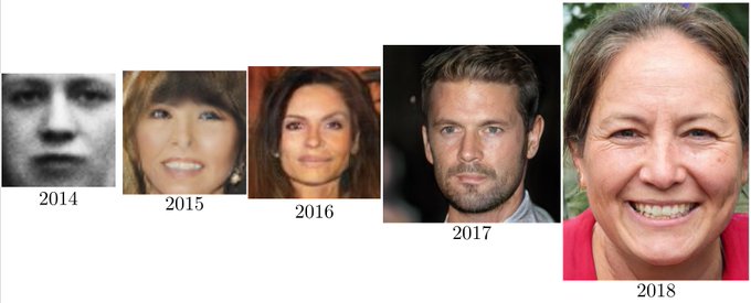
4.5 years of GAN progress on face generation.
https://arxiv.org/abs/1406.2661 https://arxiv.org/abs/1511.06434 https://arxiv.org/abs/1606.07536 https://arxiv.org/abs/1710.10196 https://arxiv.org/abs/1812.04948

— Ian Goodfellow (@goodfellow_ian)
January 15, 2019

Introduction

Oftentimes, only the most graphical Artificial Intelligence advances (image / video) are filtered out to the mainstream media. Generative Adversarial Networks (GANs) play an important role in that tip-of-the-iceberg phenomenon because they are most of the time related to images but also because they illustrate the potential of AI for creativity (e.g. https://www.thispersondoesnotexist.com/). Or at least some impression of creativity that is sufficient to blur the line between human and AI creation.

GANs have impressed the broader public with some tip-of-the-iceberg tasks such as next video frame prediction [26], image super-resolution [27], generative image manipulation (image editing and creation with minimal brush strokes) [28], introspective adversarial networks [29] (photo-editor-like features), image-to-image translation [30] (e.g. satellite images to maps, design sketches to clothing, etc.), photorealistic images from a semantic layout [31, 41] (e.g. "draw grass on the bottom, mountains in the middle and a tree in the foreground").

GANs are relatively trivial to comprehend but they are hard to tune. In addition to the complexities of GANs hyperparametrization at training time, GANs often have downstream tasks that are related to creativity and are therefore hard to benchmark. This is admittedly why several influential GAN papers remain unpublished. These elements coupled with a general authorship storm around the subject of GANs, make it difficult for the practitioner to choose the right GAN for the right purpose and to tune its hyperparameters.

This motivates the following text: an attempt at a short explanation of GANs and at producing a non-exhaustive account of the way GANs have evolved towards the most recent research iterations.

The Original Generative Adversarial Network

A generative model G creating synthetic samples is paired with a discriminative model D that estimates the probability of that synthetic data to be created by G or to be a sample of the original data. In the original GAN paper, both G and D are feedforward neural networks.

"The generative model can be thought of as analogous to a team of counterfeiters, trying to produce fake currency and use it without detection, while the discriminative model is analogous to the police, trying to detect the counterfeit currency. Competition in this game drives both teams to improve their methods until the counterfeits are indistiguishable from the genuine articles." Goodfellow et. al.

The police VS robber abalogy corresponds to a minimax game, where G aims to maximize the overlap between the distribution of the original data and the distribution of the fake data. Applying cross-entropy on point estimates is only an approximation and will be later improved upon with Wasserstein GANs (see below).

min_{G} max_{D} V (D, G) = E_{x \sim p_{d a t a} (x)} [\log D (x)] + E_{z \sim p_{z} (z)} [\log (1 - D (G (z)))]

That minimax game corresponds to a saddle point optimization problem. The optimum of the game corresponds to the Nash Equilibrium: from this point onwards, none of the two players, would benefit from a change in the players' strategies (see also image below).

(Source: Goodfellow, 2019, www.iangoodfellow.com/slides/2019-05-07.pdf.)

In practice, the minmax game is often reformulated into two loss functions:

\begin{array}{l} L_{D} = max_{D} E_{x \sim p_{d a t a} (x)} [\log D (x)] + E_{z \sim p_{z} (z)} [\log (1 - D (x))] \\ L_{G} = min_{G} E_{z \sim p_{z} (z)} [\log (1 - D (x))] \end{array}

To make it concrete, below is how one would formulate both losses in Tensorflow Keras (source):

def disc_loss(real_output, generated_output):
    bce = tf.keras.losses.BinaryCrossentropy(from_logits=True)
    return bce(tf.ones_like(real_output), real_output) + bce(
        tf.zeros_like(generated_output), generated_output
    )
def gen_loss(generated_output):
    bce = tf.keras.losses.BinaryCrossentropy(from_logits=True)
    return bce(tf.ones_like(generated_output), generated_output)

In practice, the output being a binary indicator (encoding the real / fake nature of the data), the sigmoid activation function is used. Notably, the generator loss function

min \log (1 - D (G (z)))]

) is formulated in its non-saturating form

max \log D (G (z))]

, as Goodfellow et. al. first proposed [1]. Saturation refers to the phenomenon where the optimization surface (sigmoid function here) is steep and estimates too quickly converge towards low or high extremes. At these extremes, the loss function is relatively flat and the gradient is close to zero, thus gradient descent only results in minimal steps.

While over-saturation can be controlled for (see above), several major training challenges persist:

The Helvetica scenario [1] G is trained too much without updating D. The latter is then unable to discriminate real from fake data, without G having learned to mimic the real data.
mode collapse [3]. While D converges to he correct distribution, G learns probabilities over limited modes of the original data distribution, $min_{G} max_{D} V (G, D) \neq max_{D} min_{G} V (G, D)$ [42]. It thus produces images from a certain set instead of a diversity of images (e.g. any bird created by the GAN is of the same species). Note that, in the context of creativity, it can be sometimes desirable to prioritize modes that guarantee very real-looking images over covering the entire distribution of groundtruth examples.
training a GAN corresponds to finding a Nash Equilibrium of a non-convex game with continuous high dimensional parameters. Gradient descent, as a way to find a minimum in a loss / cost function, is only a rough approximation to the Nash Equilibrium [18, 19]
D is too strong compared to G. It becomes too trivial for G to distinguish real from fake. D's gradients are close to zero and G is not provided with any more training guidance.

The last point is a lot less common [42] and is thus not a major concern in later GAN iterations. The following section summarizes the different GAN variants that either tackled these challenges or addressed new ones.

GAN Variants

In order to tackle the several challenges from the vanilla GAN above, variants of GANs have been proposed. They propose to change the loss in D or G, but also often change the architecture of the model. The descriptions below focus on GANs for images, because the most important findings emerged in that context. GANs are however capable of modeling various modalities, such as video and text, but also music (GANSynth [25]) or DNA [36].

(Most common GAN tasks, source: https://paperswithcode.com/method/patchgan)

Changes in the Loss Function

Instead of binary cross-entropy loss, some proposed to use least-square [4], f-divergence [5], hinge loss [6] and finally Wasserstein distance [7, 8, 20]. WassersteinGANs (WGANs) correct for mode collapse and for imbalances between D and G. WGANs creations also quickly became more convincing to the human eye, leading to a strong preference among researchers in the past years. In 2019, Lipschitz GANs (LGANs [51]) are shown to outperform WGANs.

While the challenges of the Helvetica scneario and mode collapse (see above) are addressed, there is little work on tackling the Nash Equilibrium condition. The game theoretical aspect is found in certain versions of WGANs [38, 39, 40].

Aside from dealing with the training challenges of GANs, other tasks emerged. Instead of the original task of distinguishing real from fake data, some proposed class prediction (CATGAN [9] or EBGAN [10] and BEGAN [11] with autoencoders) or latent representation (ALI [2], BiGAN [12], InfoGAN [13]).

Changes in the Architecture

In an attempt to build meaningful latent representations as with ALI, the original feed-forward neural network for G, can be replaced with a variational autoencoder (VAEGAN [15]). Alternatively, both D and G can be replaced by CNNs, as they are specialized at modelling images (DCGANs [17]). Later on, it is discovered that feeding patches of images as input to a GAN can sometimes outperform traditional CNN GANs (PatchGAN [16]). VEAGANs, DCGANs and PatchGANs are still very close to the original GAN in terms of the training task: creating fake images.

Quickly after its inception by Goodfellow et. al., researchers expressed the desire to see GAN perform other tasks than creation. Chronologically, the next proposed task is classification and relies on feeding auxiliary information to the network. This practice becomes known as Conditional GANs (CGANs). Multiple inputs allow CGANs to perform a multitude of tasks but can also at times improve the original creation task. Different from CGANs, where generation is conditioned on the label p(y|x), labels can also be concatenated to the data p(y,x) (e.g. ACGAN [14]). Humans found that p(y|x) and p(y,x) both outperformed the original GANs [18]. There are now three categories of models, namely GANs with no labels (unsupervised), GANs trained with labels (supervised) and CGANs trained conditioned on labels.

Other than labels, images are commonly added as conditional input to CGANs. pix2pix is the first GAN image-to-image translation network [16]. It is followed by the task of image restauration and image segmentation [43], requiring aligned training pairs. CycleGANs relax the constraint by stitching two generators head-to-toe, so that images can be translated between two sets of unpaired samples [44, 45]. UNIT architectures propose an alternative for image-to-image translation, where two VEAGANs are combined sharing the same latent space [46]. A year later, it is improved on with style attributes (MUNIT [49]).

Style-based generator architectures (StyleGANs) represent the next iteration, where an intermediary latent space is used to scale and shift the normalized image for each convolution layer [34], closely followed by StyleGAN2 in 2019 [50]. StyleGAN2 is famously capable to produce high definition images of fake individuals.

(Source: [3])

GANs Catching on Recent Trends

Given their popularity, GANs are now predominantly coupled with other recent methods. In the case where less or no labels are available, self-supervision (BigBIGAN [32]) is now prevalent. On the other hand, attention-based models attribute importance to distanced features within an image to better contextualize representation (SAGAN [33, 39]). In February 2021, in the lineage of attention-based models, transGAN proposes to discard CNNs altogether and replace them with two transformers for D and G. transGAN establishes new state-of-the-art results [52].

These recent GAN types claim the state-of-the-art in terms of performance. But performance is a non-trivial concept with GANs, as described in the following.

Evaluating GANs

While asking humans to evaluate reals from fakes seems like a sensible idea (effectively with HYPE [35]), its is a costly and time-intensive process. Alternatively, an independent critique network can be trained from scratch at GAN evaluation time to compare a holdout set of groundtruth data with the GAN generated data [22, 23, 24].

Most common non-human evaluation metrics found in recent papers claiming the state-of-the-art are Inception Score (higher is better) and Fréchet Inception Distance (lower is better) [18, 54]. Both measures are criticized for focusing on sample quality without capturing sample diversity (in other words, the metrics are not capable of detecting a mode collapse, as described above) [55, 56]. Recently, Costa et. al. proposed to measure quality diversity [21], in reaction to high-performance GANs that optimize for both quality and diversity [53].

Outlook

Over the course of this summary, we briefly formulated the original GAN and described its associated drawbacks. While the subsequent GAN iterations partly tackled these original challenges, GANs started being used for different modes (image, text, sound, video) and for different tasks (image superresolution, image style transfer, etc.). Most recently, GANs reached photo-realistic performance and was caught in the trends of transformers and self-supervision. GANs are now at a stage where a human can often not distinguish fake from real. The role of systematic quantitative GAN evaluation must be emphasized, but progress has been slower in comparison. This unbalance between creation and evaluation as a reality-check, relates to the more serious concerns of Deepfakes [57] or adversarial nets (GANs' close relatives) able to trump models and humans [58].

For further in-depth reading and learning, see the Coursera class Generative Adversarial Networks (GANs) Specialization from DeepLearning.AI (all assignments can be found here) and the book GANs in Action.

References

[1] Ian J. Goodfellow, Jean Pouget-Abadie, Mehdi Mirza, Bing Xu, David Warde-Farley, Sherjil Ozair, Aaron Courville, Yoshua Bengio: “Generative Adversarial Networks”, 2014

[2] Vincent Dumoulin, Ishmael Belghazi, Ben Poole, Olivier Mastropietro, Alex Lamb, Martin Arjovsky, Aaron Courville: “Adversarially Learned Inference”, 2016

[3] Xin Yi, Ekta Walia, Paul Babyn : "Generative adversarial network in medical imaging: A review", Medical Image Analysis, Volume 58, 2019, 101552, ISSN 1361-8415

[4] Mao, X., Li, Q., Xie, H., Lau, R.Y., Wang, Z., 2016. Least squares generative adversarial networks.

[5] Nowozin, S., Cseke, B., Tomioka, R., 2016. f-gan: Training generative neural samplers using variational divergence minimization, in: Advances in Neural Information Processing Systems, pp. 271–279.

[6] Miyato, T., Kataoka, T., Koyama, M., Yoshida, Y., 2018. Spectral normalization for generative adversarial networks.

[7] Arjovsky, M., Chintala, S., Bottou, L., 2017. Wasserstein gan.

[8] Gulrajani, I., Ahmed, F., Arjovsky, M., Dumoulin, V., Courville, A., 2017. Improved training of wasserstein gans

[9] Springenberg, J.T., 2015. Unsupervised and semi-supervised learning with categorical generative adversarial networks.

[10] Zhao, J., Mathieu, M., LeCun, Y., 2016. Energy-based generative adversarial network.

[11] Berthelot, D., Schumm, T., Metz, L., 2017. Began: boundary equilibrium generative adversarial networks.

[12] Donahue, J., Krähenbühl, P., Darrell, T., 2016. Adversarial feature learning.

[13] Xi Chen, Yan Duan, Rein Houthooft, John Schulman, Ilya Sutskever, Pieter Abbeel: “InfoGAN: Interpretable Representation Learning by Information Maximizing Generative Adversarial Nets”, 2016

[14] Odena, A., Olah, C., Shlens, J., 2016. Conditional image synthesis with auxiliary classifier gans.

[15] Larsen, A.B.L., Sønderby, S.K., Larochelle, H., Winther, O., 2015. Autoencoding beyond pixels using a learned similarity metric.

[16] Isola, P., Zhu, J.Y., Zhou, T., Efros, A.A., 2016. Image-to-image translation with conditional adversarial networks.

[17] Radford, A., Metz, L., Chintala, S., 2015. Unsupervised representation learning with deep convolutional generative adversarial networks

[18] Tim Salimans, Ian Goodfellow, Wojciech Zaremba, Vicki Cheung, Alec Radford, Xi Chen: “Improved Techniques for Training GANs”, 2016

[19] Ian J Goodfellow. On distinguishability criteria for estimating generative models. 2014

[20] David Berthelot, Thomas Schumm, Luke Metz: “BEGAN: Boundary Equilibrium Generative Adversarial Networks”, 2017

[21] Victor Costa, Nuno Lourenço, João Correia, Penousal Machado: “Exploring the Evolution of GANs through Quality Diversity”, 2020

[22] Ivo Danihelka, Balaji Lakshminarayanan, Benigno Uria, Daan Wierstra, and Peter Dayan. Comparison of Maximum Likelihood and GAN-based training of Real NVPs, 2017

[23] Daniel Jiwoong Im, He Ma, Graham Taylor, and Kristin Branson. Quantitatively Evaluating GANs With Divergences Proposed for Training, 2018

[24] Ishaan Gulrajani, Colin Raffel, and Luke Metz. Towards GAN Benchmarks Which Require Generalization, ICLR, 2019

[25] Jesse Engel and Kumar Krishna Agrawal and Shuo Chen and Ishaan Gulrajani and Chris Donahue and Adam Roberts, GANSynth: Adversarial Neural Audio Synthesis, 2019

[26] William Lotter, Gabriel Kreiman, David Cox, Deep Predictive Coding Networks for Video Prediction and Unsupervised Learning, 2017

[27] Christian Ledig, Lucas Theis, Ferenc Huszar, Jose Caballero, Andrew Cunningham, Alejandro Acosta, Andrew Aitken, Alykhan Tejani, Johannes Totz, Zehan Wang, Wenzhe Shi, Photo-Realistic Single Image Super-Resolution Using a Generative Adversarial Network, 2017

[28] Jun-Yan Zhu, Philipp Krähenbühl, Eli Shechtman, Alexei A. Efros, Generative Visual Manipulation on the Natural Image Manifold, 2018

[29] Andrew Brock, Theodore Lim, J.M. Ritchie, Nick Weston, Neural Photo Editing with Introspective Adversarial Networks, 2017

[30] Phillip Isola, Jun-Yan Zhu, Tinghui Zhou, Alexei A. Efros, Image-to-Image Translation with Conditional Adversarial Networks, 2018

[31] Taesung Park, Ming-Yu Liu, Ting-Chun Wang, Jun-Yan Zhu: “Semantic Image Synthesis with Spatially-Adaptive Normalization”, 2019, CVPR 2019

[32] Jeff Donahue, Karen Simonyan: “Large Scale Adversarial Representation Learning”, 2019

[33] Han Zhang, Ian Goodfellow, Dimitris Metaxas, Augustus Odena: “Self-Attention Generative Adversarial Networks”, 2018

[34] Tero Karras, Samuli Laine, Timo Aila: “A Style-Based Generator Architecture for Generative Adversarial Networks”, 2018

[35] Sharon Zhou, Mitchell L. Gordon, Ranjay Krishna, Austin Narcomey, Li Fei-Fei, Michael S. Bernstein, HYPE: A Benchmark for Human eYe Perceptual Evaluation of Generative Models, 2019

[36] Nathan Killoran, Leo J. Lee, Andrew Delong, David Duvenaud, Brendan J. Frey, Nathan Killoran, Leo J. Lee, Andrew Delong, David Duvenaud, Brendan J. Frey, 2017

[37] Samaneh Azadi, Catherine Olsson, Trevor Darrell, Ian Goodfellow, Augustus Odena, Discriminator Rejection Sampling, 2019

[38] Oliehoek, F.A., Savani, R., Gallego-Posada, J., Van der Pol, E., De Jong, E.D. and Gros, R., GANGs: Generative Adversarial Network Games, 2017.

[39] Oliehoek, F., Savani, R., Gallego, J., van der Pol, E. and Gross, R., Beyond Local Nash Equilibria for Adversarial Networks. 2018.

[40] Grnarova, P., Levy, K.Y., Lucchi, A., Hofmann, T. and Krause, A., An Online Learning Approach to Generative Adversarial Networks, 2017. CoRR, Vol abs/1706.03269.

[41] Taesung Park, Ming-Yu Liu, Ting-Chun Wang, Jun-Yan Zhu, Semantic Image Synthesis with Spatially-Adaptive Normalization, CVPR 2019

[42] Goodfellow, Ian, Generative Adversarial Networks (GANs), NIPS 2016 Tutorial Slides, https://www.iangoodfellow.com/slides/2016-12-04-NIPS.pdf

[43] Milletari, F., Navab, N., Ahmadi, S.A., 2016. V-net: Fully convolutional neural networks for volumetric medical image segmentation, in: 3D Vision (3DV), 2016 Fourth International Conference on, IEEE. pp. 565–571.

[44] Zhu, J.Y., Park, T., Isola, P., Efros, A.A., 2017. Unpaired image-to-image translation using cycle-consistent adversarial networks

[45] Kim, T., Cha, M., Kim, H., Lee, J.K., Kim, J., 2017. Learning to discover cross-domain relations with generative adversarial networks.

[46] Liu, M.Y., Breuel, T., Kautz, J., 2017a. Unsupervised image-to-image translation networks, in: Advances in Neural Information Processing Systems, pp. 700–708.

[49] Xun Huang, Ming-Yu Liu, Serge Belongie, Jan Kautz: “Multimodal Unsupervised Image-to-Image Translation”, 2018

[50] Tero Karras, Samuli Laine, Miika Aittala, Janne Hellsten, Jaakko Lehtinen, Timo Aila: “Analyzing and Improving the Image Quality of StyleGAN”, 2019

[51] Zhiming Zhou, Jiadong Liang, Yuxuan Song, Lantao Yu, Hongwei Wang, Weinan Zhang, Yong Yu, Zhihua Zhang: “Lipschitz Generative Adversarial Nets”, 2019

[52] Yifan Jiang, Shiyu Chang, Zhangyang Wang: “TransGAN: Two Transformers Can Make One Strong GAN”, 2021

[53] Andrew Brock, Jeff Donahue, Karen Simonyan: “Large Scale GAN Training for High Fidelity Natural Image Synthesis”, 2018

[54] M. Heusel, H. Ramsauer, T. Unterthiner, B. Nessler, G. Klambauer, S. Hochreiter. GANs Trained by a Two Time-Scale Update Rule Converge to a Nash Equilibrium, CoRR, Vol abs/1706.08500. 2017.

[55] S. Barratt, R. Sharma., A Note on the Inception Score, 2018.

[56] I. Gulrajani, C. Raffel, L. Metz., Towards GAN Benchmarks Which Require Generalization, International Conference on Learning Representations. 2019.

[57] Thanh Thi Nguyen, Cuong M. Nguyen, Dung Tien Nguyen, Duc Thanh Nguyen, Saeid Nahavandi: “Deep Learning for Deepfakes Creation and Detection: A Survey”, 2019

[58] Yang, L., Song, Q. & Wu, Y. Attacks on state-of-the-art face recognition using attentional adversarial attack generative network. Multimed Tools Appl 80, 855–875 (2021).

Generative Adversarial Networks