A Story About Transfer Learning

A common belief is that deep learning was popularized when AlexNet won the ImageNet competition. Indeed AlexNet was a huge breakthrough, but something else played a very important role, too.

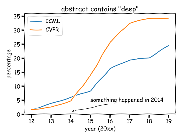
To understand the hidden factors, I analyzed CVPR (a top-tier conference for computer vision) and ICML (a top-tier conference for machine learning). I calculated the proportion of papers whose abstract contain the word “deep”, from 2012 to 2019.

Prior to 2012, just a few papers (basically from Hinton's group) mentioned "deep". After AlexNet in 2012, the percentage started to go up. However, few people noticed that, there is another turning point in 2014, when the percentage started to grow rapidly.

What happened in 2014? After a literature survey, I believe the following papers played an important role:

Rich feature hierarchies for accurate object detection and semantic segmentation, CVPR 2014, citation over 1.5w
Decaf: A deep convolutional activation feature for generic visual recognition, ICML 2014, citation over 4k

The first paper is the RCNN paper, which demonstrated that features from pre-trained AlexNet could greatly benefit object detection and semantic segmentation. The second paper demonstrated that features from pre-trained AlexNet could benefit generic visual classification problems. Both of them extended the power of pre-trained AlexNet to downstream tasks, showing how deep neural networks can be transferred to benefit broad tasks.

Therefore, transfer learning is the hidden force behind deep learning.

The Status Quo of Transfer Learning

When we talk about transfer learning, we mean the practice of fine-tuning pre-trained models to a new target dataset.

The fine-tuning pipeline (in the figure below) is extremely simple. In computer vision, practitioners often choose an ImageNet pre-trained model, remove the last fully connected layer, add a randomly initialized layer, and then start fine-tuning. Intuitively, the last fully-connected layer is task-specific, and cannot be reused in a new task. So the status quo of transfer learning is simply to copy pre-trained weight as initialization.

It is straightforward to copy the weight of bottonm layers. But, can we further re-use the top fc layer? Actually, after counting the percentage of parameters in the discarded fc layer, I found that they took up a decent amount of total parameters! For popular NLP models like BERT, the fc layer can take up to 21% of total parameters!

Re-use the Discarded FC Layer to Improve Transfer Learning

I will directly dive into the code implementation to explain the idea behind the paper. A figure is also available in the below to illustrate the procedure.

Say we have an input dataset

{x_{i}}_{i = 1}^{n}

. By feeding the dataset into a pre-trained model (

F_{\bar{θ}}

), we can get features

{f_{i}}_{i = 1}^{n}

. Typically this is the end of transfer learning: the final fc layer (

G_{θ_{s}}

) of the pre-trained model is discarded and the features are fed into a randomly initialized fc layer (

H_{θ_{t}}

) to get predictions

{{\hat{y}}_{i}^{t}}_{i = 1}^{n}

(we use subscript/superscript "t" to denote target dataset, and use "s" to denote the source/pre-training dataset). Then the labels from target dataset

{y_{i}^{t}}_{i = 1}^{n}

can supervise the predictions to calculate the loss function needed for training neural networks. That's the whole story of naive fine-tuning.

Since we notice that

G_{θ_{s}}

takes a large proportion of parameters, we propose a way to re-use

G_{θ_{s}}

First, we can feed the features

{f_{i}}_{i = 1}^{n}

into

G_{θ_{s}}

to get output

{{\hat{y}}_{i}^{s}}_{i = 1}^{n}

. The target prediction

{{\hat{y}}_{i}^{t}}_{i = 1}^{n}

is supervised by the target labels

{y_{i}^{t}}_{i = 1}^{n}

, then how about the source prediction

{{\hat{y}}_{i}^{s}}_{i = 1}^{n}

? In the common case of ImageNet pre-trained models, the output space of

{\hat{y}}^{s}

is a 1000-class categorical distribution. Therefore, if somehow we figure out a 1000-dimentional vector to supervise ${y_{i}^{t}}_{i = 1}^{n}$ , we can re-use the previously discarded fc layer!

How to find the supervision? It seems very difficult, but remember we have target label

{y_{i}^{t}}_{i = 1}^{n}

for each data point, therefore we can convert the target label

y^{t}

into another form

y^{s}

to supervise the output

{{\hat{y}}_{i}^{s}}_{i = 1}^{n}

for another branch

G_{θ_{s}}

! The conversion is shown as the "Category Relationship" in the figure, and is easy to calculate despite the scary formula in the paper. Actually, it only requires 7 lines! See the below code.

def category_relationship(pretrain_prob, target_labels):
    """
    The direct approach of learning category relationship.
    :param pretrain_prob: shape [N, N_p], where N_p is the number of classes in pre-trained dataset
    :param target_labels:  shape [N], where 0 <= each number < N_t, and N_t is the number of target dataset
    :return: shape [N_c, N_p] matrix representing the conditional probability p(pre-trained class | target_class)
     """
    N_t = np.max(target_labels) + 1 # the number of target classes
    conditional = []
    for i in range(N_t):
        this_class = pretrain_prob[target_labels == i]
        average = np.mean(this_class, axis=0, keepdims=True)
        conditional.append(average)
    return np.concatenate(conditional)

That said, the procedure of Co-Tuning is very simple:

Feed the target dataset into the pre-trained model, collect the target labels and probabilistic outputs from the pre-trained model.
Calculate the category relationship relationship=category_relationship(pretrain_prob, target_labels) by the above code.
Use simple indexing y_s = relationship[y_t] to get the "label" for the output of $G_{θ_{s}}$ .

This is a simplified version of my NeurIPS 2020 paper Co-Tuning for Transfer Learning. For more details, check the paper yourself or check the code repository https://github.com/thuml/CoTuning. The paper contains many sophisticated techniques to further improve Co-Tuning, but I think this post is enough for readers to get the main idea.

Experimental Results

We present parts of the experimental results in the below. Compared to baseline fine-tune (naive transfer learning), the Co-Tuning method can greatly improve the classification performance, especially when the proportion of available data (sampling rates) is small.

In Stanford Cars dataset with sampling rate of 15%, baseline fine-tuning accuracy is 36.77% and Co-Tuning improves the accuracy to 46.02%, bringing in up to 20% relative improvement!

Reference

Co-Tuning for Transfer Learning, NeurIPS 2020

Co-Tuning: An easy but effective trick to improve transfer learning

A Story About Transfer Learning

The Status Quo of Transfer Learning

Re-use the Discarded FC Layer to Improve Transfer Learning

Experimental Results

Reference

Recommended for you

Co-Tuning: An easy but effective trick to improve transfer learning

A Story About Transfer Learning

The Status Quo of Transfer Learning

Re-use the Discarded FC Layer to Improve Transfer Learning

Experimental Results

Reference

Recommended for you

Report Article